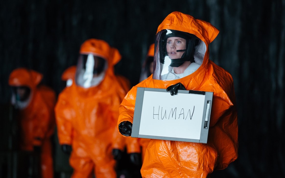
How would YOU communicate with Aliens ? How would you teach them your language ? The way we teach children right ? By showing them pictures of various objects and their names.
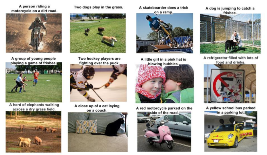
Basically Associating the Image and the Text. That’s the goal of automatic image captioning.
It is an extensive topic and decades of research has gone into cracking this problem. A blog post can never do justice to this field just as reading the caption is not the same as looking at the picture! But one can try.
If you just want to use a general image captioning system, you should be happy to know that google has open sourced their system and made it available under im2txt repo in TensorFlow. If you use torch/lua, then NeuralTalk2 by Karpathy would be a good starting point as the code is available on github. You must know however, that Google has done much more engineering to make it suitable for real world usage, so TensorFlow is more recommended way to go.
In this post, we will describe the foundation upon which these current SOAs’ in image captioning are based. While we are reaching human level performance in many problem domains( e.g. image classification, speech recognition, face verification). However, automatic image captioning, even after decades of research hasn’t come close to human level performance. But the surge of deep learning in object recognition, localization and fine-grained attribute identification has led to an unprecedented boost in the accuracy of relatively hard computer vision problem of image captioning. Earlier methods involved transferring the most relevant description from indexed database by finding the semantically similar images through image retrieval. Obviously, their applicability was limited.
Current image captioning methodologies can be divided into three categories:
- The first set of methods detect objects and attributes and then piece together a description for the image from the phrases containing those objects.
- The second set of methods embed images and corresponding captions in the same vector space. For a given query, captions nearest to the image in the embedding space are retrieved and those captions are modified to generate a new caption for the given image. However, these methods do not generate a novel description of a given test image as the descriptions from the most similar images are used to spur out the caption.
- The third set of methods directly generate the sequence of the words most relevant to the image conditioned on the image and previously generated words. Therefore, they can produce novel combinations of words that might never have occurred in the training data. This has become the standard pipeline in most of the state of the art algorithms for image captioning and is described in a greater detail below.Let’s deep dive:
Recurrent Neural Networks(RNNs) are the key
For the task of image captioning, a model is required that can predict the words of the caption in a correct sequence given the image. This can be modeled as finding the caption that maximizes the following log probability.
$$\log p(S|I) = \sum_{t=0}^{N} \log p(S_{t}|I,S_{0},S_{1}……S_{t-1}) \hspace{2cm} (eqn : 1)$$
where:
- \(S\) is the caption,
- \(S_{t}\) is the word in the caption at location t (\(t_{th}\) word)
The probability of a word depends on the previously generated words and the image, and hence the conditioning on these variables in the equation. The training data consists of thousands of images and a caption associated with each image. The captions in the training data is written by humans. The training phase involves finding the parameters in the model that maximizes the probability of captions given the image in the training set.
In probabilistic graphical models, for this type of densely connected node variables wherein every node is dependent on all other nodes, training becomes computationally prohibitive because of an exponential number of possible configurations. Recurrent Neural Networks (RNN) provide a smooth way to perform the conditioning on previous variables using a fixed sized hidden vector.
This hidden vector is then used to predict the next word just like a feed forward neural network.
$$p(S_{t}|I,S_{0},S_{1}……..S_{t-1}) \approx p(S_{t}|I,h_{t}) \hspace{2cm} (eqn : 2)$$
So at the step t, the complex conditioning on a variable number of nodes is replaced by a simple vector(\(h_{t}\)). Then for making the prediction at step t, eqn:2 is used to model the probability distribution over all the words using a fully connected layer with number of outputs as number of words in vocabulary followed by softmax function. So \(p(S_{t}|I,h_{t})\) becomes
$$p(S_{t}|I,h_{t}) = softmax(L_{h}h_{t}+L_{I}I)$$
Where \(L_{h}\) and \(L_{I}\) are the weight matrices of the fully connected layer with inputs taken as one concatenated vector from \(h_{t}\) and I.
According to this distribution, the word with maximum probability is taken as the next word in the caption. Now at the step t+1, the conditioning on the previously generated words should also involve this newly generated word(\(S_{t}\)). But the RNN vector(\(h_{t}\)) is conditioned on the words \(S_{1}, S_{2} …. S_{t-1}\). So \(S_{t}\) is then combined with \(h_{t}\) through a linear layer followed by a non-linearity to produce \(h_{t+1}\) which stands for conditioning on \(S_{1}, S_{2} …. S_{t-1}, S_{t}\) . This is called an RNN unit which comprises of this calculation:
$$h_{t+1}=tanh(W_{h}h_{t}+W_{s}S_{t}) \hspace{2cm} (eqn : 3)$$
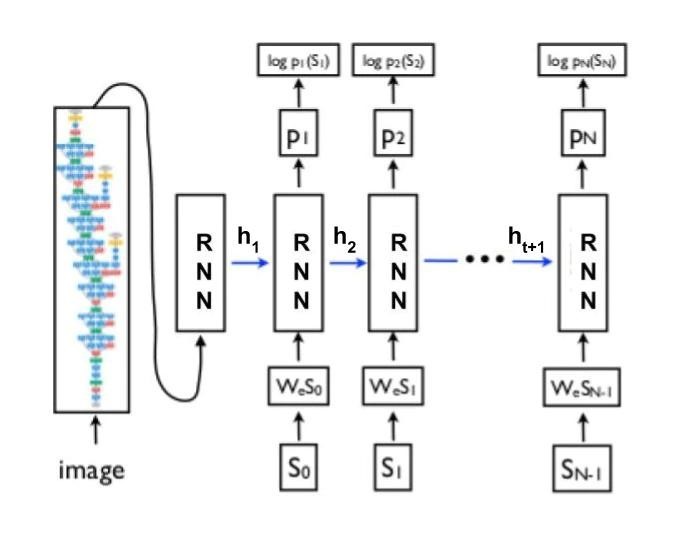
Figure : 2
The overall flow of the algorithm has been shown in figure 2.
Since RNN is basically like the conventional feed forward neural comprising of linear and non-linear layers, the back-propagation of loss during training is straight-forward without performing heavy inference computations. The only difference with a normal neural network is that the clubbing of the previous hidden vector and newly generated word is done through the same set of parameters at each step. This is equivalent to feeding the output to the same network as input and hence the name recurrent neural network. This avoids blowing up the size of the network which otherwise would require a new set of parameters at each step. The RNN unit can be represented as shown in figure 3.
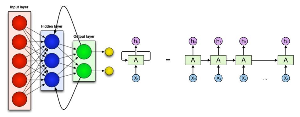
Figure : 3
Before we move forward, let me explain a very important concept in machine learning. Typically, we want to represent everything ( images, sounds, words etc. ) as a vector ( i.e. an array of numbers ). You can also think of this vector of length n as a point in an n-dimensional space. But why represent images and words as vectors ? Because we understand vector spaces and we understand distances in vector spaces. E.g. we know that the point (1,0,0) is closer to the point (0,0,0) than the point (0,5,0) in three dimensional space. If we could represent two words by points in a higher dimensional space, we could easily calculate how close they are in meaning or context by just calculating the distance of these points in higher dimensional space.
Conceptually, representing images and words as points in higher dimensional space sounds wonderful. The hard part is to figure out how to do this.
The image is represented as a vector by taking the penultimate layer (before the classification layer) output from any of the standard convolutional networks viz. VGGnet, GoogleNet etc.
For words, we want the representation should be such that the vectors for the words similar in meaning or context should lie close to each other in the vector space. An algorithm that converts a word to a vector is called word2vec and it is arguably the most popular one. word2vec draws inspiration from the famous quote “You shall know the word from the company it keeps” to learn the representation for words.
Learning of word2vec is done using a corpus ( psst… this is a fancy word for “collection of text” ) of sentences related to the domain in which we are working. Let’s use the domain “computer vision” as an example. Let \(w_{1},w_{2} ……w_{M}\) be the unique words in the corpus and \(S_{w_{1}},S_{w_{2}} …..S_{w_{M}}\) be the corresponding word vector that we need to find. In order to determine the word vectors, word2vec trains a system that can predict the surrounding words of a given word. Surrounding words are defined as words appearing around a given word in a small context window of a given size (let’s say 2 here) on both sides of that word. Let these three sentences be our corpus. ( This is just for demonstration purposes; in real world applications, the size of the corpus should be very large to get a meaningful representation.)
This blog is about deep learning and computer vision.
We love deep learning.
We love computer vision.
Given a word “computer”, the task is to predict the context words “learning”, “and” and “vision” from first sentence and “we”, “love” and “vision” from last sentence. Therefore the training objective becomes maximising the log probability of these context words given the word “computer”. The formulation is:
$$Objective = Maximize \sum_{t=1}^{T} \sum_{-m\geq j \geq m} log P (S_{w_{t+j}} | S_{w_{t}})$$
where:
m : is the context window size (here 2) and t runs over the length of the corpus (i.e. every word in the collection of sentences)
\( P(S_{w_{t+j}}|S_{w_{t}}) \) is modelled by the similarity or inner product between the context word vector and center word vector. For each word there are two vectors associated with it viz. when it appears as context and when it is the center word represented by R and S respectively.
So \(P(S_{w_{t+j}}|S_{w_{t}})\) is taken as \(\frac{e^{R_{w_{t+j}}^{T}}}{\sum_{i=1}^{M} e^{R_{i}^{T}S_{w_{t}}}}\). Here denominator is the normalization term that takes the similarity of center word vector with the context vectors of every other word in vocabulary so that probability sums to one.
The center vector for a word is then taken as the vector representation and is used with the RNN in eqn: 3.
Dealing with noise in real world images: Attention Mechanism
When there is clutter in the scene it becomes very difficult for simpler systems to generate a complex description of the image. We, humans, do it by getting a holistic picture of the image at first glance. Our focus then shifts to different regions in the image as we go on describing the image. For machines, a similar attention mechanism has been proposed to mimic human behavior. This attention mechanism allows only important features from an image to come to the forefront when needed. At each step, the salient region of the image is determined and is fed into the RNN instead of using features from the whole image. The system gets a focused view from the image and predicts the word relevant to that region. The region where attention is focussed needs to be determined on the basis of previously generated words. Otherwise, newly generated words may be coherent within the region but not in the description being generated.
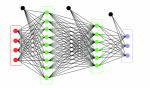
Until now the output of the fully connected layer was used as input to the RNN. This output corresponds to the entire image. So, how do we get a feature corresponding to only a small subsection of the image ? The output of the convolutional layer encodes local information and not the information pertaining to the whole cluttered image. The outputs of the convolutional layer are 2d feature maps where each location was influenced by a small region in the image corresponding to the size (receptive field) of the convolutional kernel. To understand this have a look at the figure 4(as shown in wikipedia page of convolutional network) which shows a convolutional network. Just before the output layer, there is a fully connected layer which is like one stretched vector and stands for the whole input image whereas the convolutional layer outputs(all the layers before the fully connected one) are like a 2d image with many dimensions. The vector extracted from a single feature map at a particular location and across all the dimensions signify the feature for a local region of the image.
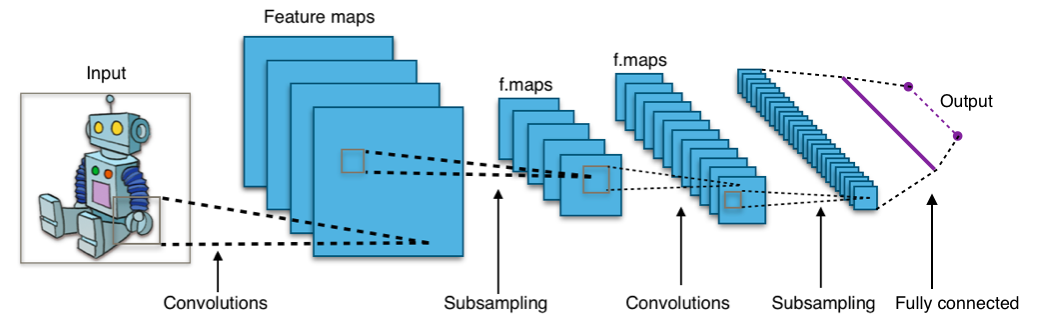
Figure: 4
At each step, we want to determine the location on the feature map that is relevant to the current step. The feature vector from this location will be fed into the RNN. So we model the probability distribution over locations based on previously generated words. Let \(L_{t}\) be a random variable with n dimensions with each value corresponding to a spatial location on feature map. \(L_{t,i} = 1\) means the \(i_{th}\) location is selected for generating the word at the t step. Let \(a_{i}\) be the feature vector at the \(i_{th}\) location taken from convolutional maps.
The value we need is:
$$p(L_{t,i} = 1 | I,S_{0},S_{1}……..S_{t-1}) \approx p(L_{t,i}|h_{t}) = \beta_{t,i} \propto a_{i}^{T}h_{t} \hspace{1cm}(eqn:4)$$
Here probability of choosing a location (\(\beta_{t,i}\)) has been taken as directly proportional to the dot product i.e. similarity between vector at that location and the RNN hidden vector.
Now on the basis of probability distribution, the feature vector corresponding to the location with the maximum probability can be used for making the prediction, but using an aggregated vector from all the location vectors weighted according to the probabilities makes the training converge simply and fastly. So let the \(z_{t}\) be the context or aggregated vector which is to be fed into the RNN.
$$z_{t} = \sum_{i=1}^n\beta_{t,i}a_{i}$$
So the eqn:2 becomes
$$p(S_{t}|I,h_{t}) => p(S_{t}|z_{t},h_{t})$$
So this mechanism simulate the human behavior of focusing their attention to various parts of the image while describing it and naturally with the focused view, a more sophisticated description can be generated for the image which caters to even the finer level details in the image. Figure 5 shows one of the examples given in the Reference 1.
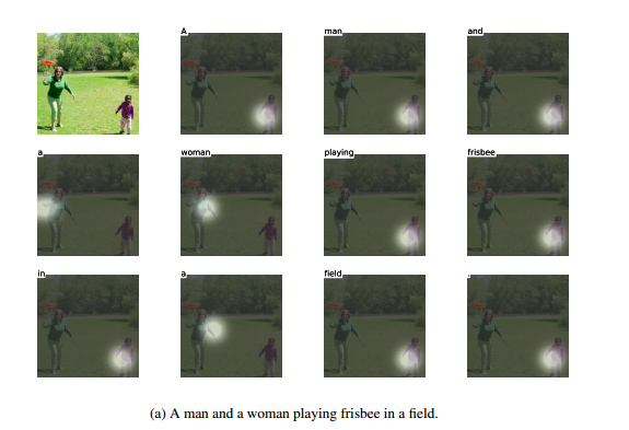
Figure : 5
All these small components are like bedrock for most prevalent image captioning systems nowadays. There are many papers for image captioning with most of them working around these central ideas and between those papers, most of the changes are more or less in these areas:
- How the word vectors are learned.(ex. Glove is another methodology to generate word vectors)
- Backpropagation to be done on image and word2vec layers or not.
- LSTM(long short term memory) used in place of RNN which takes care of vanishing gradient problem in RNN.
- Stochastic vs soft attention: Here we have discussed soft attention mechanism wherein different location vectors are aggregated on the basis of their individual probabilities. In the stochastic mechanism, a single location is sampled on the basis of probability distribution and vector from just that location is used in the RNN unit.
References:
- Xu, J. Ba, R. Kiros, A. Courville, R. Salakhutdinov, R. Zemel, and Y. Bengio, Show, attend and tell: Neural image caption generation with visual attention
- Vinyals, A. Toshev, S. Bengio, and D. Erhan, Show and tell: A neural image caption generator