Image Segmentation using deconvolution layer in Tensorflow

In this series of post, we shall learn the algorithm for image segmentation and implementation of the same using Tensorflow. This is the first part of the series where we shall focus on understanding and be implementing a deconvolutional/fractional-strided-convolutional layer in Tensorflow.

Why is deconvolutional layer so important?

Image segmentation is just one of the many use cases of this layer. In any type of computer vision application where resolution of final output is required to be larger than input, this layer is the de-facto standard. This layer is used in very popular applications like Generative Adversarial Networks(GAN), image super-resolution, surface depth estimation from image, optical flow estimation etc. These are some direct applications of deconvolution layer. It has now also been deployed in other applications like fine-grained recogntion, object detection. In these use cases, the existing systems can use deconvolution layer to merge responses from different convolutional layers and can significantly boosts up their accuracy.

There are 4 main parts of this post:

1. What is image segmentation?

2. What is deconvolutional layer?

3. Initialization strategy for deconvolutional layer.

4. Writing a deconvolutional layer for Tensorflow.

Let’s get started.

1. What is Image Segmentation?

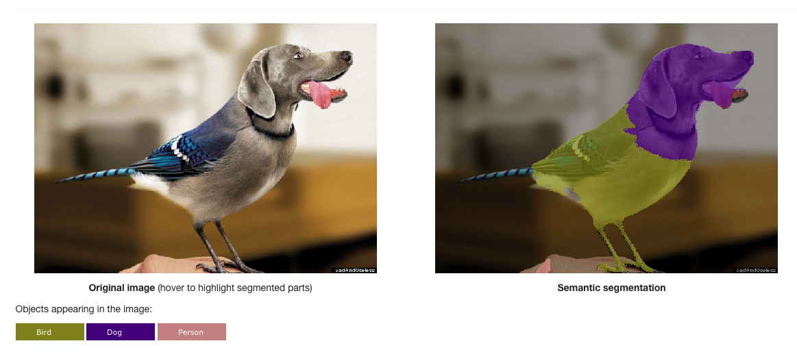
Image segmentation

image segmentation is the process of dividing an image into multiple segments(each segment is called super-pixel). And each super-pixel may represent one common entity just like a super-pixel for dog’s head in the figure. Segmentation creates a representation of the image which is easier to understand and analyze as shown in the example. Segmentation is a computationally very expensive process because we need to classify each pixel of the image.

Convolutional neural networks are the most effective way to understand images. But there is a problem with using convolutional neural networks for Image Segmentation.

But, How to use convolutional neural networks for image segmentation:

In general, CNN performs down-sampling, i.e. they produce output of lower resolution than the input due to the presence of max-pool layer. Look at the figure below: This shows alexnet and size at each layer. It’s fed an image of 224*224*3=150528 and after 7 layers, we get a vector of size 4096. This is the representation of the input image that’s great for image classification and detection problems.

alexnet network architecture: tensorflow tutorial

However, since segmentation is about finding the class of each and every pixel of the image, down-sampled maps cannot be directly used. For this, we use an upsampling convolutional layer which is called deconvolutional layer or fractionally strided convolutional layer.

2. What is Fractionally Strided convolution or deconvolution?

Fractionally strided convolution/deconvolution layer upsamples the image to get the same resolution as the input image. A simple resizing of the maps is an option as we do for resizing of an image. But since a naive upsampling inadvertently loses details, a better option is to have a trainable upsampling convolutional layer, whose parameters will change during training.

So, for image segmentation, a deconvolutional layer is put on top of regular CNN. The down-sampled response maps from CNN are upsampled through this deconvolution layer, producing the feature that can be used to predict class labels at all the pixel locations. These predictions are compared with the ground truth segmentation labels available, and a loss function is defined which guides the network towards correct prediction by updating the parameters involved in backward propagation as usual.

The general intuition is that deconvolution is a transformation that goes in the opposite direction of normal convolution, hence the name. So in deconvolution, output of convolution becomes the input of deconvolution and input of convolution becomes output of deconvolution.

2.1 Detailed understanding of fractionally strided convolution/deconvolution:

In order to understand how this operation can be reverted, let’s first take an example of convolution with 1-D input. First we shall look at the normal convolution process and later we shall reverse the operation to develop an understanding of the corresponding deconvolutional operation.

Figure 1

Suppose:

x: 1-D input arranged in an array.

y: output array of convolution.

Kernel size: 4 (figure 1)

Stride: 2

Kernel size being 4 means there are 4 different weights depicted with indices 1,2,3,4 as shown in figure 1.

The convolution process is depicted in figure 2 wherein filter slides horizontally across x(top) to produce output y(left). As usual, to get the output, weights at each location are multiplied with corresponding input and summed up. And since the stride is 2, the output map is just half the resolution of input map.

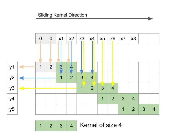
The arrows in the figure, indicate what all x are used to compute a y. Look at it carefully, each y depends on 4 consecutive x. So here, y2 depends only on x1, x2, x3, x4 which is indicated by blue coloured arrows. Similarly dependency of y3 is shown by yellow coloured arrows so on and so forth.

FIGURE 2: Depiction of usual convolution process with 1-D input

Now, let’s reverse these operations.

In order to flip the input and output, we will first reverse the direction of arrows from figure 2 to obtain the figure 3. Now the input is y and the output is x. Let’s see how the inputs and outputs are related.

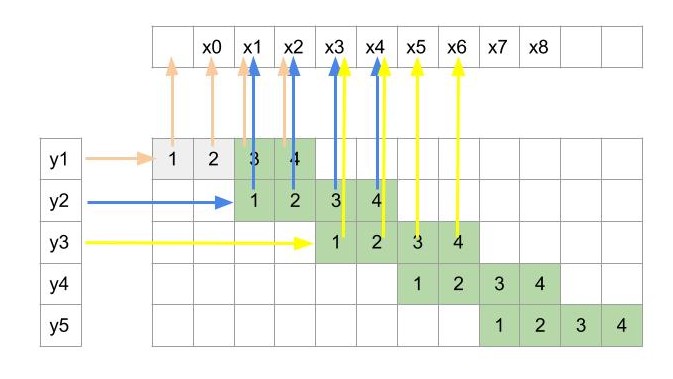
Figure 3: Reversing the data-flow in convolution

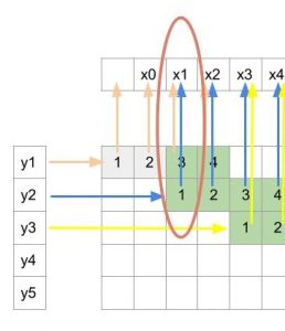
Figure 4

Since y2 was obtained from x1 to x4 during convolution, so here y2 will be an input for only those 4 x’s i.e. x1 to x4. Similarly, y3 will be input for x3 to x6. So, each y will have the contribution towards 4 consecutive x.

Also from the arrows, we can see that x1 depends only on y1 and y2(pointed in figure 4). Similarly, x2 also depends only on y1 and y2. So each output x here depends only on two consecutive inputs y whereas in the previous convolution operation the output was dependent on 4 inputs.

Figure 5 shows what all inputs(y) are used to compute an output(x).

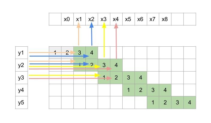
Figure 5: Shows what all inputs(y) are used to compute an output(x)

This obviously is very different from normal convolution. Now the big question is, can this operation be cast as a convolution operation wherein a kernel is slid across y(vertically in our case as y is arranged vertically) to get output x.

From the figure 5 we can see x1 is calculated using only kernel indices 3 and 1. But x2 is calculated using indices 4 and 2. This can be thought as two different kernels are active for different outputs which is different from the regular convolution where a single kernel is used throughout for all the outputs. Here one kernel is responsible for outputs at x1, x3, x5 …x2k-1 and other kernel produces x2, x4 …. x2k. The problem with carrying out the operation in this way is that it’s very inefficient. The reason is that we will first have to use one kernel for producing outputs at odd numbered pixels and then use other kernel for even numbered pixels. Finally we will have to stitch these different sets of outputs by arranging them alternately to get final output.

We will now see a trick which can make this process efficient.

Lets put one void value(zero) between every two consecutive y. We obtain figure 6. Here we have not changed any connectivity between x and y. Each x depends on the same set of y’s and two newly inserted zeros. Since zeros do not change the summation, we still have the same operation. But the beauty of this little tweak is that each x now uses the same single kernel. We do not need to have two different sets of kernels. A single kernel with size 4 can be slide across y to get the same output x. Since x is twice the resolution of y, we now have a methodology to increase the resolution.

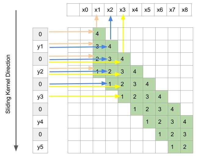
Figure 6: Depiction of fractionally strided convolution

So a deconvolution operation can be performed in the same way as a normal convolution. We just have to insert zeros between the consecutive inputs and define a kernel of an appropriate size and just slide it with stride 1 to the get the output. This will ensure an output with a resolution higher than the resolution of its inputs. The general rule is to insert as many zeros between successive inputs as the increase in the resolution requires, subtracted by 1. This ensures that for each pixel, (scale_factor – 1) pixels are newly produced. So, if 2x is required, we insert 1 zero and similarly, if 3x is required, 2 zeros are inserted. The fractionally strided convolution name stems from this fact that, inserting zeros between elements effectively introduces a convolution with the stride 1/n, where n is the factor of increase in resolution.

An added benefit with this operation is that since weights are associated with operation and that too in a linear way(multiplying and adding), we can easily back-propagate through this layer.

So, hopefully this gives you detailed understanding and intuition for a fractionally strided convolutional layer. In the next step, we shall cover the initialization of this layer.

3. Initialization of fractionally strided convolution layer:

The performance of a deep neural network is heavily impacted by the way layers are initialized. So let’s look into the details for initialization of deconvolutional layer.

We discussed earlier that the concept of a deconvolution operation stems from the concept of upsampling of features which resembles bilinear interpolation. So it makes sense that the idea for initialization of the layers is heavily inspired and designed such that it can perform a bilinear interpolation.

So, let’s first understand the normal upsampling just like a regular image resizing.

3.1 Image Upsampling:

There are just four pixels in an image as shown in figure(red dots). We term these as original pixels. The pixel value is denoted by alphabet O in the figure, and the task is to perform 3x upsampling. This amounts to inserting 2 pixels between the successive pixel locations denoted in gray. The value of the pixel which is newly inserted is denoted by the alphabet N in the figure.

FIGURE 7

In bilinear interpolation, the value of the newly inserted pixel is calculated by interpolating values from nearest pixels for which values are already known. The ratio of contribution taken from the pixels is inversely proportional to the ratio of corresponding distance.

So value N1 is calculated by interpolating O1 and O2 on the basis of its distance from those pixels. N1 is 1-pixel distance from O1 and 2-pixel distance from O2. Therefore,

contrib_O1/contrib_O2 = 2/1

Also, the total contribution from both pixels should sum up to 1. With some algebraic manipulation, we can see that

contrib_O1 = 2/3, and

contrib_O2 = 1/3.

Similarly for N2, the contribution is 1/3 and 2/3, respectively.

Now the question is, how does this bilinear interpolation relate to a convolutional kernel?

3.2 How to use this for deconvolutional layer initialization?

Let’s have a convolutional kernel of size 5 for the same example.

FIGURE 8

Let us put the kernel such that its center is on the pixel, N1. When this kernel is convolved, the value N1 is obtained by the weighted sum of the input values. In order to replicate the effect of bilinear interpolation, the weight corresponding to O1 and O2 location is taken as 2/3 and 1/3, respectively. So let’s put these values in the kernel at the appropriate locations(indices).

FIGURE 9

Similarly, keeping the center of the kernel at N2, the weights are filled up from the bilinear weights calculated.

Lastly, for the center located at O2, the weight is 1 because its value is already known.

FIGURE 10

So, now we have a kernel of size 5 with the weights such that when convolved with the input image, it performs a bilinear interpolation.

In tensorflow, it can be carried out as below.

def get_bilinear_filter(filter_shape, upscale_factor):
        ##filter_shape is [width, height, num_in_channels, num_out_channels]
        kernel_size = filter_shape[1]
        ### Centre location of the filter for which value is calculated
        if kernel_size % 2 == 1:
            centre_location = upscale_factor - 1
        else:
            centre_location = upscale_factor - 0.5

bilinear = np.zeros([filter_shape[0], filter_shape[1]])
        for x in range(filter_shape[0]):
            for y in range(filter_shape[1]):
                ##Interpolation Calculation
                value = (1 - abs((x - centre_location)/ upscale_factor)) * (1 - abs((y - centre_location)/ upscale_factor))
                bilinear[x, y] = value
        weights = np.zeros(filter_shape)
        for i in range(filter_shape[2]):
            weights[:, :, i, i] = bilinear
        init = tf.constant_initializer(value=weights,
                                       dtype=tf.float32)

bilinear_weights = tf.get_variable(name="decon_bilinear_filter", initializer=init,
                               shape=weights.shape)
        return bilinear_weights

def get_bilinear_filter(filter_shape, upscale_factor):

##filter_shape is [width, height, num_in_channels, num_out_channels]

kernel_size = filter_shape[1]

### Centre location of the filter for which value is calculated

if kernel_size % 2 == 1:

centre_location = upscale_factor - 1

else:

centre_location = upscale_factor - 0.5

bilinear = np.zeros([filter_shape[0], filter_shape[1]])

for x in range(filter_shape[0]):

for y in range(filter_shape[1]):

##Interpolation Calculation

value = (1 - abs((x - centre_location)/ upscale_factor)) * (1 - abs((y - centre_location)/ upscale_factor))

bilinear[x, y] = value

weights = np.zeros(filter_shape)

for i in range(filter_shape[2]):

weights[:, :, i, i] = bilinear

init = tf.constant_initializer(value=weights,

dtype=tf.float32)

bilinear_weights = tf.get_variable(name="decon_bilinear_filter", initializer=init,

shape=weights.shape)

return bilinear_weights

With this understanding, let us see how to make a deconvolutional layer in tensorflow.

4. Writing fractionally strided convolutional layer in Tensorflow :

Let’s say we have an input feature map with the number of channels as n_channels, and the upscale_factor be the increase in the resolution we require from the layer. Let the input tensor going into the layer be termed as input.

Tensorflow has an inbuilt module for deconvolutional layer called tf.nn.conv2d_transpose. It takes in the arguments just like a convolutional layer with a notable exception that transpose layer requires the shape of the output map as well. The spatial extent of the output map can be obtained from the fact that (upscale_factor –1 ) pixels are inserted between two successive pixels.

The “strides” input argument is little different from a convolutional layer. Since the stride is a fraction in deconvolutional layer, it is taken as the stride for the convolutional operation. That is, basically the stride of the equivalent convolutional kernel which can revert the effect of deconvolutional layer. So stride in x and y direction is simply the location difference between O1 and O2 in the figure 5 ie. upscale_factor.

Weights are initialized from bilinear interpolation and can be obtained from the function mentioned earlier.

The following snippet of code takes the input tensor “bottom” and puts a deconvolutional layer on top of it.

def upsample_layer(bottom,

n_channels, name, upscale_factor):

kernel_size = 2*upscale_factor - upscale_factor%2

stride = upscale_factor

strides = [1, stride, stride, 1]

with tf.variable_scope(name):

# Shape of the bottom tensor

in_shape = tf.shape(bottom)

h = ((in_shape[1] - 1) * stride) + 1

w = ((in_shape[2] - 1) * stride) + 1

new_shape = [in_shape[0], h, w, n_channels]

output_shape = tf.stack(new_shape)

filter_shape = [kernel_size, kernel_size, n_channels, n_channels]

weights = get_bilinear_filter(filter_shape,upscale_factor)

deconv = tf.nn.conv2d_transpose(bottom, weights, output_shape,

strides=strides, padding='SAME')

return deconv

So, we have covered the most important part for implementing segmentation in Tensorflow. In the follow up post, we shall implement the complete algorithm for image segmentation and will see some results.

deconvolution, Image segmentation, transpose convolution layer