MOTR is a state of the art end-to-end multiple object tracker that does not require any temporal association between objects of adjacent frames. It directly outputs the track of objects in a sequence of input images (video). MOTR uses Deformable DETR for object detection on a single image. To understand the architecture of MOTR it is useful to start with the its object detection method ie. Deformable DETR. But since Deformable DETR just uses the DETR architecture with the attention module replaces by a Multi-Scale Deformable Attention (MSDA) module, it would be helpful to first study DETR.
DETR is a recent state of the art SOTA architecture for end-to-end object detection from Facebook AI. It is different from the previous two stage object detection architectures. The previous two stage architectures consists of classification and regression stages. Region Proposal Net (RPN) is used for generating region proposal in the first stage. Afterwards, classification and regression processes are performed. R-CNN, Fast R-CNN and Faster R-CNN are the most well-known algorithms of this architecture.
DETR
The DETR architecture consists of two layers:
- CNN backbone layer
- Transformer layer

DETR architecture
The first layer processes the input image using a CNN backbone. It produces features for the input image. These feature maps are then fed into the transformer layer to generate bounding box, class, and class confidence scores for a fixed number of predictions. This number, N, is chosen to be much larger than the typical number of objects in an image to make sure that the bounding boxes corresponding to all objects can be predicted.
Once we have the predicted bounding boxes, we use a bi-partite matching algorithm to match the predicted boxes to the ground truth objects. Since the number of predictions would be larger than the number of ground truth objects, we use a special “no object” class in the predictions to make sure a valid one-to-one matching between the ground truth objects and predictions can exist. The loss is then calculated using this bi-partite matching.
The bi-partite matching is calculated by minimizing the following metric:

where \({\frak{S}}_N\) denotes the set of all permutation functions on natural number 1 to N, \(\hat{y}_i\) denotes the \(i^{th}\) prediction \((\hat{b}_i, \{\hat{p}_i(c_j)\}_{j=1}^N)\) from the neural network and \(y_i = (b_i, c_i)\) denotes the ground truth. The metric \(\cal{L}_{match}(y_i, \hat{y}_{\sigma(i)})\) is defined as \( -\mathfrak{1}_{\{c_i \ne \emptyset \}} \hat{p}_{\sigma(i)}(c_i) + \mathfrak{1}_{\{c_i \ne \emptyset \}} \cal{L}_{box}(b_i, \hat{b}_{\sigma(i)}) \), where \(\cal{L}_{box }()\) is the bounding box loss. This optimal assignment is then computed using the Hungarian algorithm. After finding the bi-partite matching the loss function of the NeuraNet can be calculated as,

Many different models can be used for the CNN backbone in Layer 1. The DETR paper uses ResNet-50 and ResNet-101. For layer 2 a transformer layer is used as follows:

Transformer Layer in DETR
Transformer Encoder: First a 1×1 convolution operation is used to reduce the dimensions of the input feature map from the CNN backbone, creating a new feature map of dimension \(\mathbb{R}^{dxHxW}\) with height H and width W. We flatten this input to an input of size \(\mathbb{R}^{dxHW}\) and use 2D positional encodings to encode this input.
Transformer Decoder: The decoder follows the standard architecture of the transformer. But one difference with the original transformer is that our model decodes the N objects in parallel at each decoder layer, while Vaswani et al.‘s transformer predicts the output sequence one element at a time. The embeddings input into the decoder are learnable parameters referred to as object queries. These object queries are treated as learnable positional encoding and added to the input of each attention layer, like in the encoder.
The output of the transformer decoder is then independently decoded into box coordinates and class labels. The box coordinates are predicted by a feed forward network, a 3-layer perceptron with ReLU activation function and hidden dimension d. A linear layer predicts the class label using a softmax function.
Auxillary Loss: The authors use auxiliary losses in decoder during training, especially to help the model output the correct number of objects of each class. FFNs and Hungarian loss are added after each decoder layer. All predictions FFNs share their parameters. We use an additional shared layer-norm to normalize the input to the prediction FFNs from different decoder layers.
Let us now look at the MSDA attention module used to replace the attention layer in DETR.
Multi-Scale Deformable Attention Module (MSDA)
The MSDA can be described more easily by looking at the deformable attention module and then generalising the architecture to MSDA.
Deformable Attention Module: The deformable attention module is inspired by deformable convolution. It is helpful in reducing the computational complexity of the attention module. In a normal attention module the query pay attention to all the keys which creates an unnecessary computational overhead for the attention layer. In deformable attention the queries are given a fixed budget of keys to pay attention to, and the key coordinates are taken as learnable parameters of the model.
The output of the deformable attention layer, for query vector \(\mathbf{z}_q\) corresponding to position position \(\mathbf{p}_q\) and input feature map \( \mathbf{x} \in \mathbb{R}^{C x H x W}\), can now be described as follows:

where K is the fixed budget of keys to pay attention to, M is the number of heads, \(A_{mqk} \) is the attention for head m, query q and key k, and \(A_{mqk}\) denotes the attention weight of the \(k^{th}\) sampling point in the \(m^{th}\) attention head. \( \Delta \mathbf{p}_{mqk} \) corresponds to the learned offset in the key coordinates chosen in the budget.
The position \( \mathbf{p}_q + \Delta\mathbf{p}_{mqk} \) can fall in between pixels. So, a bilinear interpolation is used to compute \( \mathbf{x}(\mathbf{p}_q + \Delta\mathbf{p}_{mqk}) \).
Multi-Scale Deformable Attention: The proposed Deformable Attention module is naturally extendable to multi-scale feature maps obtained from the CNN backbone.
Let \( \{ \mathbf{x}^l \}_{l=1}^L\) be the multi-scale feature maps for \(\mathbf{x}^l \in \mathbb{R}^{CxH_lxW_l}\) and \( \hat{\mathbf{p}}_q\) denote the coordinates of the reference point, then with notation similar to Deformable Attention module, we can write the output of MSDA as follows:

where \( \phi_l (\hat{\mathbf p}_q)\) re-scales the coordinates to the input feature map of the l-th level.
Now by replacing the transformer attention modules — i.e. the self attention in encoder and the cross attention in the decoder– with deformable attention modules in DETR, we can construct Deformable DETR.
MOTR : Multi-Object Tracking with tRansformers
MOTR is a simple online tracker. It is easy to develop based on DETR with minor modifications on label assignment.
MOTR modifies the object query input in DETR to track queries, which corresponds to tracks of objects in a video. It does that with the following architecture:

MOTR architecture
MOTR processes each frame of a video using Deformable DETR. The object queries in DETR are extended to track queries, used to keep track of sequence of object detections in each frame. The decoder is input a fixed length set of object queries –referred to as detect queries in this paper– corresponding to new born objects, and a variable length set of track queries corresponding to tracked objects.
The label assignment for detect queries is done via bipartite matching with new born objects, similar to DETR. While the track queries follow the same assignment of previous frames. The Query Interaction Module (QIM) is desgined as follows:

QIM
The QIM takes as input the hidden state produced by the transformer decoder, and the track queries from the previous frame. The filtered hidden states corresponding to the persisting track queries is passed through the Temporal Aggregation Network (TAN). The output of TAN is then concatenated with the hidden state for detect queries corresponding to newborn objects to form the track queries for the next frame.
During training, the detect queries are filtered based on the assignment of new born objects according to the bi-partite matching algorithm. The track queries are filtered by removing the exited objects from them based on if the object disappered in the ground truth or if the intersection-over-union (IoU) between predicted bounding box and target is below a threshold of 0.5.
During inference, we use predicted classification scores to determine appearance of newborn objects and disappearance of tracked objects. For object queries, predictions whose classification scores are higher than the entrance threshold \(\tau_{en}\) are kept while other hidden states are removed. For track queries, predictions whose classification scores are lower than the exit threshold \(\tau_{ex}\) for consecutive M frames are removed while other hidden states are kept.
The TAN is a modified Transformer decoder layer. It works to enhance temporal relation modeling and provide contextual priors for tracked objects.
MOTR Inference Demo
To run the inference on the MOTR, git clone the MOTR repository as follows: git clone https://github.com/megvii-research/MOTR. Now, inside the MOTR folder create a Dockerfile with the following:
|
1 2 3 4 5 6 7 8 9 10 11 12 13 14 15 16 17 18 19 20 21 22 23 24 |
ARG CUDA=11.7.1 ARG CUDNN=8 ARG UBUNTU=20.04 FROM nvidia/cuda:${CUDA}-cudnn${CUDNN}-devel-ubuntu20.04 ENV TZ=Asia/Dubai RUN ln -snf /usr/share/zoneinfo/$TZ /etc/localtime && echo $TZ > /etc/timezone RUN apt-get update RUN apt-get install ffmpeg libsm6 libxext6 build-essential git vim wget -y RUN apt-get install software-properties-common -y RUN add-apt-repository ppa:deadsnakes/ppa RUN apt install python3.7 python3.7-dev pip python3.7-distutils -y RUN yes | python3.7 -m pip install torch torchvision torchaudio COPY requirements.txt ./ RUN yes | python3.7 -m pip install -r requirements.txt RUN yes | python3.7 -m pip install gdown RUN update-alternatives --install /usr/bin/python3 python3 /usr/bin/python3.7 10 RUN update-alternatives --install /usr/bin/python python /usr/bin/python3.7 10 |
Build and run the docker with the following commands:
docker build -t motr .

docker run -it --name motr --gpus all --shm-size 24G -v $PWD:$PWD motr
Now compile the MSDA library with the following:
cd models/ops

./make.sh
Download the MOTR model path with the following command: gdown https://drive.google.com/uc?id=1K9AbtzTCBNsOD8LYA1k16kf4X0uJi8PC. Now run the following command to run the demo:
|
1 2 3 4 5 6 7 8 9 10 11 12 13 14 15 16 17 18 19 20 21 22 23 24 25 26 27 |
EXP_DIR=exps/e2e_motr_r50_joint python3 demo.py \ --meta_arch motr \ --dataset_file e2e_joint \ --epoch 200 \ --with_box_refine \ --lr_drop 100 \ --lr 2e-4 \ --lr_backbone 2e-5 \ --pretrained model_motr_final.pth \ --output_dir ${EXP_DIR} \ --batch_size 1 \ --sample_mode 'random_interval' \ --sample_interval 10 \ --sampler_steps 50 90 120 \ --sampler_lengths 2 3 4 5 \ --update_query_pos \ --merger_dropout 0 \ --dropout 0 \ --random_drop 0.1 \ --fp_ratio 0.3 \ --query_interaction_layer 'QIM' \ --extra_track_attn \ --resume model_motr_final.pth \ --input_video figs/demo.avi |
PS: To make the repo work you might have to comment the version comparison code in MOTR/util/misc.py (lines 32-61)