In this post, I shall explain object detection and various algorithms like Faster R-CNN, YOLO, SSD. We shall start from beginners’ level and go till the state-of-the-art in object detection, understanding the intuition, approach and salient features of each method.
What is Image Classification?:
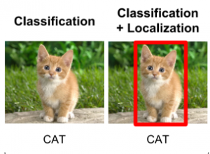
Image classification takes an image and predicts the object in an image. For example, when we built a cat-dog classifier, we took images of cat or dog and predicted their class:

What do you do if both cat and dog are present in the image:

What would our model predict? To solve this problem we can train a multi-label classifier which will predict both the classes(dog as well as cat). However, we still won’t know the location of cat or dog. The problem of identifying the location of an object(given the class) in an image is called localization. However, if the object class is not known, we have to not only determine the location but also predict the class of each object.
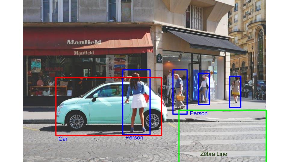
Predicting the location of the object along with the class is called object Detection. In place of predicting the class of object from an image, we now have to predict the class as well as a rectangle(called bounding box) containing that object. It takes 4 variables to uniquely identify a rectangle. So, for each instance of the object in the image, we shall predict following variables:
class_name,
bounding_box_top_left_x_coordinate,
bounding_box_top_left_y_coordinate,
bounding_box_width,
bounding_box_height
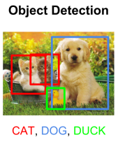
Just like multi-label image classification problems, we can have multi-class object detection problem where we detect multiple kinds of objects in a single image:
In the following section, I will cover all the popular methodologies to train object detectors. Historically, there have been many approaches to object detection starting from Haar Cascades proposed by Viola and Jones in 2001. However, we shall be focussing on state-of-the-art methods all of which use neural networks and Deep Learning.
Object Detection is modeled as a classification problem where we take windows of fixed sizes from input image at all the possible locations feed these patches to an image classifier.

Demo of Sliding WIndow detector
Each window is fed to the classifier which predicts the class of the object in the window( or background if none is present). Hence, we know both the class and location of the objects in the image. Sounds simple! Well, there are a few more problems. How do you know the size of the window so that it always contains the image? Look at examples:
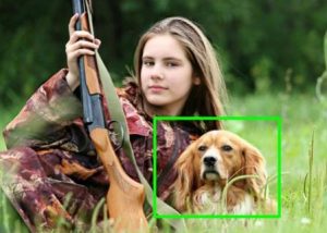
Small sized object
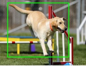
Big sized object. What size do you choose for your sliding window detector?
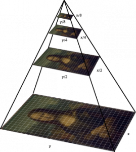
As you can see that the object can be of varying sizes. To solve this problem an image pyramid is created by scaling the image.Idea is that we resize the image at multiple scales and we count on the fact that our chosen window size will completely contain the object in one of these resized images. Most commonly, the image is downsampled(size is reduced) until certain condition typically a minimum size is reached. On each of these images, a fixed size window detector is run. It’s common to have as many as 64 levels on such pyramids. Now, all these windows are fed to a classifier to detect the object of interest. This will help us solve the problem of size and location.
There is one more problem, aspect ratio. A lot of objects can be present in various shapes like a sitting person will have a different aspect ratio than standing person or sleeping person. We shall cover this a little later in this post. There are various methods for object detection like RCNN, Faster-RCNN, SSD etc. Why do we have so many methods and what are the salient features of each of these? Let’s have a look:
1. Object Detection using Hog Features:
In a groundbreaking paper in the history of computer vision, Navneet Dalal and Bill Triggs introduced Histogram of Oriented Gradients(HOG) features in 2005. Hog features are computationally inexpensive and are good for many real-world problems. On each window obtained from running the sliding window on the pyramid, we calculate Hog Features which are fed to an SVM(Support vector machine) to create classifiers. We were able to run this in real time on videos for pedestrian detection, face detection, and so many other object detection use-cases.
2. Region-based Convolutional Neural Networks(R-CNN):
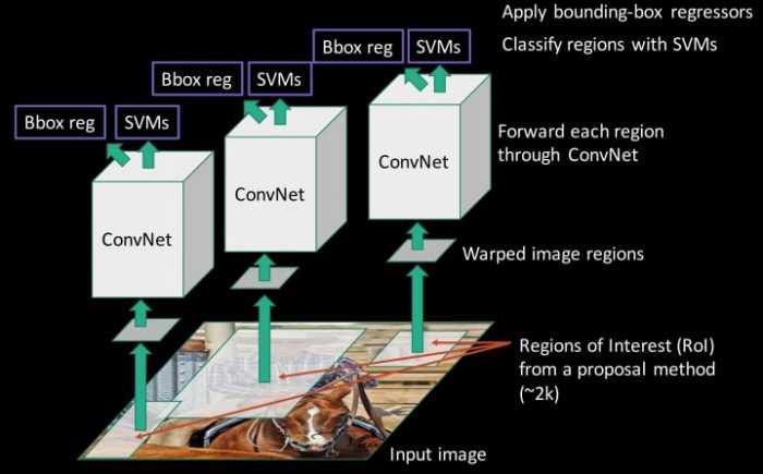
Since we had modeled object detection into a classification problem, success depends on the accuracy of classification. After the rise of deep learning, the obvious idea was to replace HOG based classifiers with a more accurate convolutional neural network based classifier. However, there was one problem. CNNs were too slow and computationally very expensive. It was impossible to run CNNs on so many patches generated by sliding window detector. R-CNN solves this problem by using an object proposal algorithm called Selective Search which reduces the number of bounding boxes that are fed to the classifier to close to 2000 region proposals. Selective search uses local cues like texture, intensity, color and/or a measure of insideness etc to generate all the possible locations of the object. Now, we can feed these boxes to our CNN based classifier. Remember, fully connected part of CNN takes a fixed sized input so, we resize(without preserving aspect ratio) all the generated boxes to a fixed size (224×224 for VGG) and feed to the CNN part. Hence, there are 3 important parts of R-CNN:
- Run Selective Search to generate probable objects.
- Feed these patches to CNN, followed by SVM to predict the class of each patch.
- Optimize patches by training bounding box regression separately.
3. Spatial Pyramid Pooling(SPP-net):
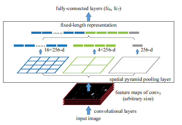
Still, RCNN was very slow. Because running CNN on 2000 region proposals generated by Selective search takes a lot of time. SPP-Net tried to fix this. With SPP-net, we calculate the CNN representation for entire image only once and can use that to calculate the CNN representation for each patch generated by Selective Search. This can be done by performing a pooling type of operation on JUST that section of the feature maps of last conv layer that corresponds to the region. The rectangular section of conv layer corresponding to a region can be calculated by projecting the region on conv layer by taking into account the downsampling happening in the intermediate layers(simply dividing the coordinates by 16 in case of VGG).
There was one more challenge: we need to generate the fixed size of input for the fully connected layers of the CNN so, SPP introduces one more trick. It uses spatial pooling after the last convolutional layer as opposed to traditionally used max-pooling. SPP layer divides a region of any arbitrary size into a constant number of bins and max pool is performed on each of the bins. Since the number of bins remains the same, a constant size vector is produced as demonstrated in the figure below.
However, there was one big drawback with SPP net, it was not trivial to perform back-propagation through spatial pooling layer. Hence, the network only fine-tuned the fully connected part of the network. SPP-Net paved the way for more popular Fast RCNN which we will see next.
4. Fast R-CNN:
Fast RCNN uses the ideas from SPP-net and RCNN and fixes the key problem in SPP-net i.e. they made it possible to train end-to-end. To propagate the gradients through spatial pooling, It uses a simple back-propagation calculation which is very similar to max-pooling gradient calculation with the exception that pooling regions overlap and therefore a cell can have gradients pumping in from multiple regions.
One more thing that Fast RCNN did that they added the bounding box regression to the neural network training itself. So, now the network had two heads, classification head, and bounding box regression head. This multitask objective is a salient feature of Fast-rcnn as it no longer requires training of the network independently for classification and localization. These two changes reduce the overall training time and increase the accuracy in comparison to SPP net because of the end to end learning of CNN.
5. Faster R-CNN:
So, what did Faster RCNN improve? Well, it’s faster. And How does it achieve that? Slowest part in Fast RCNN was Selective Search or Edge boxes. Faster RCNN replaces selective search with a very small convolutional network called Region Proposal Network to generate regions of Interests.
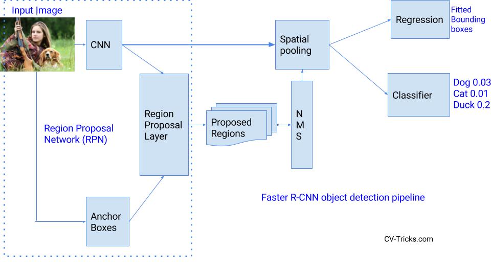
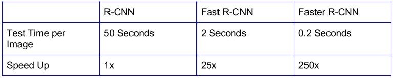
To handle the variations in aspect ratio and scale of objects, Faster R-CNN introduces the idea of anchor boxes. At each location, the original paper uses 3 kinds of anchor boxes for scale 128x 128, 256×256 and 512×512. Similarly, for aspect ratio, it uses three aspect ratios 1:1, 2:1 and 1:2. So, In total at each location, we have 9 boxes on which RPN predicts the probability of it being background or foreground. We apply bounding box regression to improve the anchor boxes at each location. So, RPN gives out bounding boxes of various sizes with the corresponding probabilities of each class. The varying sizes of bounding boxes can be passed further by apply Spatial Pooling just like Fast-RCNN. The remaining network is similar to Fast-RCNN. Faster-RCNN is 10 times faster than Fast-RCNN with similar accuracy of datasets like VOC-2007. That’s why Faster-RCNN has been one of the most accurate object detection algorithms. Here is a quick comparison between various versions of RCNN.
Regression-based object detectors:
So far, all the methods discussed handled detection as a classification problem by building a pipeline where first object proposals are generated and then these proposals are send to classification/regression heads. However, there are a few methods that pose detection as a regression problem. Two of the most popular ones are YOLO and SSD. These detectors are also called single shot detectors. Let’s have a look at them:
6. YOLO(You only Look Once):
For YOLO, detection is a simple regression problem which takes an input image and learns the class probabilities and bounding box coordinates. Sounds simple?
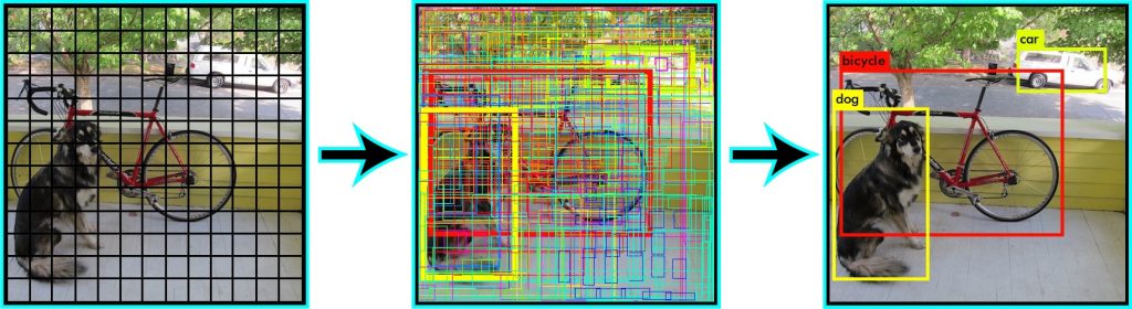
YOLO divides each image into a grid of S x S and each grid predicts N bounding boxes and confidence. The confidence reflects the accuracy of the bounding box and whether the bounding box actually contains an object(regardless of class). YOLO also predicts the classification score for each box for every class in training. You can combine both the classes to calculate the probability of each class being present in a predicted box.
So, total SxSxN boxes are predicted. However, most of these boxes have low confidence scores and if we set a threshold say 30% confidence, we can remove most of them as shown in the example below.
Notice that at runtime, we have run our image on CNN only once. Hence, YOLO is super fast and can be run real time. Another key difference is that YOLO sees the complete image at once as opposed to looking at only a generated region proposals in the previous methods. So, this contextual information helps in avoiding false positives. However, one limitation for YOLO is that it only predicts 1 type of class in one grid hence, it struggles with very small objects.
7. Single Shot Detector(SSD):
Single Shot Detector achieves a good balance between speed and accuracy. SSD runs a convolutional network on input image only once and calculates a feature map. Now, we run a small 3×3 sized convolutional kernel on this feature map to predict the bounding boxes and classification probability. SSD also uses anchor boxes at various aspect ratio similar to Faster-RCNN and learns the off-set rather than learning the box. In order to handle the scale, SSD predicts bounding boxes after multiple convolutional layers. Since each convolutional layer operates at a different scale, it is able to detect objects of various scales.
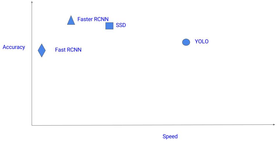
That’s a lot of algorithms. Which one should you use? Currently, Faster-RCNN is the choice if you are fanatic about the accuracy numbers. However, if you are strapped for computation(probably running it on Nvidia Jetsons), SSD is a better recommendation. Finally, if accuracy is not too much of a concern but you want to go super fast, YOLO will be the way to go. First of all a visual understanding of speed vs accuracy trade-off:
SSD seems to be a good choice as we are able to run it on a video and the accuracy trade-off is very little. However, it may not be that simple, look at this chart that compares the performance of SSD, YOLO, and Faster-RCNN on various sized objects. At large sizes, SSD seems to perform similarly to Faster-RCNN. However, look at the accuracy numbers when the object size is small, the gap widens.
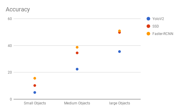
YOLO vs SSD vs Faster-RCNN for various sizes
Choice of a right object detection method is crucial and depends on the problem you are trying to solve and the set-up. Object Detection is the backbone of many practical applications of computer vision such as autonomous cars, security and surveillance, and many industrial applications. Hopefully, this post gave you an intuition and understanding behind each of the popular algorithms for object detection.