Prologue:This is a three part series which will elaborate on Object Detection in images using Convolutional Neural Networks (CNN). First part will deal with groundbreaking papers in detection. Second part will give an overview on some of the fancier methodologies that have been published recently. Third part will be about one of our more sophisticated methods in performing detection in a domain like fashion where context around the regions play an important role. By the time I started writing this post, I came across two papers which deal with the context in a much different way than what we devised. So I will discuss those too.
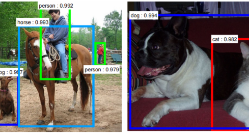
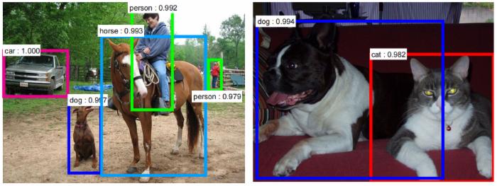
An image classification problem is predicting the label of an image among the predefined labels. It assumes that there is single object of interest in the image and it covers a significant portion of image. Detection is about not only finding the class of object but also localizing the extent of an object in the image. The object can be lying anywhere in the image and can be of any size(scale) as can be seen in the figure 1.
So object classification is no more helpful when:
- Multiple objects in image
- Objects are small
- Exact location and size of object in image is desired
Traditional methods of detection involved using a block-wise orientation histogram(SIFT or HOG) feature which could not achieve high accuracy in standard datasets such as PASCAL VOC. These methods encode a very low level characteristics of the objects and therefore are not able to distinguish well among the different labels. Deep learning (Convolutional networks) based methods have become the state
of the art in object detection in image. They construct a representation in a hierarchial manner with increasing order of abstraction from lower to higher levels of neural network. Starting from Girshick et. al. paper, a flurry of papers have been published which have either focused on improving run-time efficiency or accuracy. These have used more or less the same pipeline involving CNN(convolutional neural network)as feature extractor. This post will try to cover salient points in some of the most influential works in this direction.
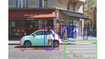
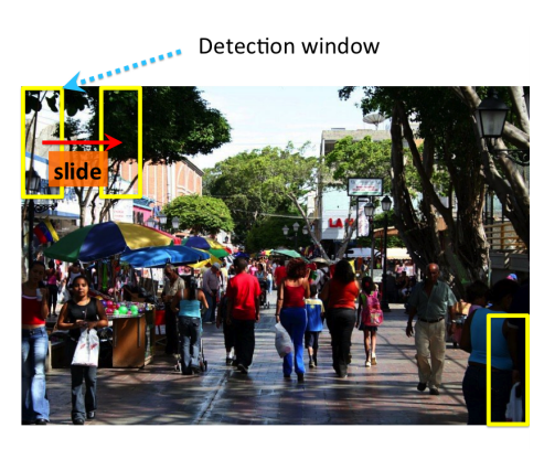
One could perform detection by carrying out a classification on different sub-windows or patches or regions extracted from the image. The patch with high probability will not only the class of that region but also implicitly gives its location too in the image. Most of the approaches vary on the type of methodology used for choosing the windows. One brute force method is to run classification on all the sub-windows formed by sliding different sized patches(to cover each and every location and scale) all through the image as in the figure 2.
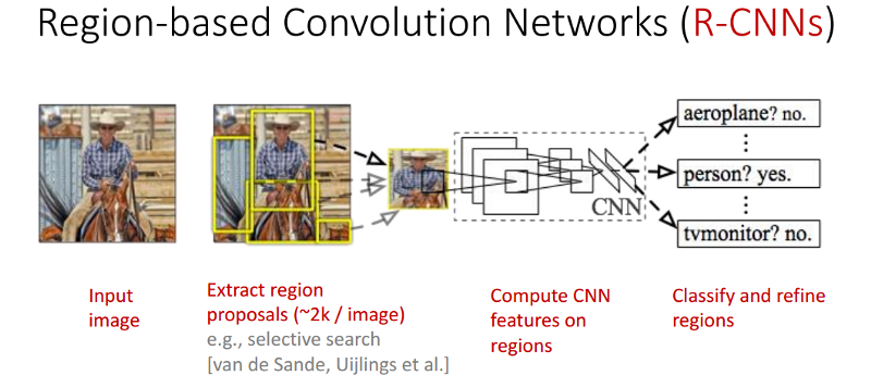
As you may have guessed it right, this will be a tedious process from computational time point of view as each sub-window would require passing it through CNN and calculating the feature for that region. R-CNN therefore uses a object proposal algorithm like selective search(SS) in its pipeline which gives out a number(~2000) of TENTATIVE object locations and extents on the basis of local cues like color rgb, hsv etc. This does not use any fancy supervised algorithm and therefore is class-agnostic which can be used independent of the domain. These object regions are warped to a fixed sized(227X227) pixels and are fed to a classification convolutional network which gives the individual probability of the region belonging to background and classes. The tricky part is feeding the appropriate regions labeled as background during the training of convolutional network. If random regions that do not have anything to do with the object classes are fed as background the network wont be able to distinguish between the object regions and regions which are partially containing the objects. Therefore regions which have an IOU greater than 0.5 with the objects are marked with class of that object and those with overlap < 0.3 are marked as background. As in the classification training, SGD is used to train the network end to end. The second stage of RCNN involves improving the localization(coordinates of the extent of object) accuracy by minimizing the error of predicted coordinates against the ground truth coordinates. This is required because SS need not necessarily produces regions which can encompass the objects perfectly. For this a linear regression layer is optimized on top of Conv5 layer after fine-tuning the network for classification. Since this training is done independent of classification training, conv5 layer and layers preceding it cannot be finetuned once their weights have been optimized for classification(because we will be using the same network for both to reduce computation time). In the test time an additional technique NMS(non maximal suppresion) is used to merge highly overlapping regions which are predicted to be of same class.
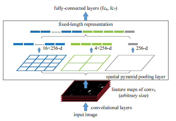
SPP(spatial pyramid pooling) is one of the turning points for making a highly accurate RCNN pipeline feasible in run-time. RCNN had to pass all the ~2000 regions from SS independently through CNN and is therefore a very slow algorithm. SPP allows the whole image(not individual regions but the whole image) to be passed through the convolutional layer only once. This saves a lot of time because same patch may belong to multiple regions and convolutions on them are not calculated multiple time as done in RCNN thereby enabling a shared computation of conv layers among the regions. Since major chunk of time(~90%) is spent on the convolutional layers it reduces the computation time drastically. After passing the image through conv layers, independent feature need to be calculated for each of the regions generated by SS. This can be done by performing a pooling type of operation on JUST that section of the feature maps of last conv layer that corresponds to the region. The rectangular section of conv layer corresponding to a region can be calculated by projecting the region on conv layer by taking into account the downsampling happening in the intermediate layers(simply dividing the coordinates by 16 in case of VGG). Normally a max pooling layer follows the final conv layer of CNN, but the feature vector produced by max pool layer depends upon the size of region(3X3 max pool with stride 1 on 5X5 maps would produce 3X3 output while on 7X7 would give 5X5 output) and therefore vector obtained cannot be fed into the following FC layers which require a fixed sized vector as input. SPP solves this problem by replacing max pooling layer with spatial pooling layer. SPP layer divides a region of any arbitrary size into constant number of bins and max pool is performed on each of the bins. Since number of bins remain the same, a constant size vector is produced as demonstrated in the figure 4 below. The training windows for positive and negative samples are chosen in the same manner as RCNN. The only difference in SPP net is that since windows of arbitrary size are used for pooling operation, back-propagation through SPP layer and finetuning the network end-to-end is not trivial and therefore SPP net finetunes just FC part of the network and gradients are not propagated across the SPP layer. The second part follows on the same lines as RCNN wherein it fits a linear regression layer for localization on top of conv5 layers.
Still SPP has certain downsides that it does not use the full potential of CNN because training is not end-to-end. Fast RCNN tackles the downsides by installing the net with the capacity to back-propagate the gradients from FC layer to conv. layers. It is a simple back-propagation calculation and is very similar to max-pooling gradient calculation with the exception that pooling regions overlap and therefore a cell can have gradients pumping in from multiple regions. Second major change is a single network with two loss branches pertaining to soft-max classification and bounding box regression. This multitask objective is a salient feature of Fast-rcnn as it no longer requires training of the network independently for classification and localization. These two changes reduces the overall training time and increases the accuracy in comparision to SPP net because of end to end learning of CNN.
In the pipeline of fast-rcnn, the slowest part is generating regions from selective search SS(~2s) or edgeboxes(~0.2s). Faster-RCNN replaces SS with CNN itself for generating the region proposals(called RPN-region proposal network) which gives out tentative regions at almost negligible amount of time. This is done by using the convolutional layers from detection network(therefore no overhead) and introducing two convolutional layers on top of this (in parallel to FC layers of detection network) to generate regions at various spatial location. Since the conv layers are shared it does not add to the computation time and the only additional time involved is the two additional conv layers which have relatively small number of filters. So for RPN a small network with kernel size of 3X3 is run through the final conv feature map and a smaller 256 dimension feature is obtained at every spatial location. This is then fed to the two sibling layers just as in previous detection network for the two tasks of classification and localization. Since the task of RPN is to generate potential object like regions classification layer has only two outputs for background and foreground. Its like sliding the window across the feature map. This small layer takes in fixed number(3X3) of pixels for making the prediction about the coordinates of objects which can be of any size or aspect ratio. And therefore different sets of parameters are used for different sizes and aspect ratio. In the following figure three sets of sizes and three sets of aspect ratio(square, vertically elongated and horizontally elongated) are used. These are called anchor boxes and are centered at the sliding window location. So for these 9 anchor boxes(k), a total of 36(9k) is the number of outputs for regression layer encoding 4 coordinates for each anchor box and 18(2k) outputs for classification layer that gives an estimate of the probabilities of object or not object for each box. The anchor box having the highest overlap with the ground truth box is labeled as an object. Also the boxes having a high overlap percentage(>0.7) are also marked as foreground. All the anchor boxes with overlap percentage < 0.3 are labeled as background.
Training bit is a little tricky and different from previous methods because RPN and Detection network when trained independently would set different weights for conv layers which would defeat the purpose of shared conv layers for reducing computation time. Therefore authors proposed an alternating approach as follows. First RPN is trained and regions obtained are used to train detection network. Then RPN is retrained but this time with the conv part initialized with weights from conv part of detection network. In this run ,only the newly added conv layers(not being used in detection network) are finetuned for RPN and this makes the conv layers to have the same weights as detection network. Finally the new RPN is used to generate the regions and fed to the training for detection network in which only the FC layers are finetuned. This is a like alternating optimization used in optimization problem involving two variables when fixing one variable converts the problem into an easy to optimize function dependent on second variable.

All these methods concentrate on increasing the run-time efficiency of object detection without compromising on the accuracy. Faster-Rcnn has become a state-of-the-art technique which is being used in pipelines of many other computer vision tasks like captioning, video object detection, fine grained categorization etc.
References:
- Ross Girshick, Jeff Donahue, Trevor Darrell, Jitendra Malik: Rich feature hierarchies for accurate object detection and semantic segmentation
- Kaiming He, Xiangyu Zhang, Shaoqing Ren, Jian Sun: Spatial Pyramid Pooling in Deep Convolutional Networks for Visual Recognition
- Ross Girshick: Fast R-CNN
- Shaoqing Ren, Kaiming He, Ross Girshick, Jian Sun: Faster R-CNN: Towards Real-Time Object Detection with Region Proposal Networks
- http://www.cs.utoronto.ca/~fidler/slides/CSC420/lecture17.pdf