It’s no news that Deep Learning is super effective and powerful in solving computer vision problems. To keep things in perspective, the top 5 accuracy of NASnet on the ImageNet dataset is 96.2% which is greater than human accuracy on the same task(approx 94.9%). Similarly, deep learning has surpassed or equaled the human level accuracy for most of the tasks. Hence, these models are being widely used in a number of fields like Medicine, Surveillance, Defence etc. However, despite being extremely accurate, these Deep Learning models are highly vulnerable to attacks. In this post, we shall discuss what are adversarial examples and how they can be used to break machine learning systems.
What are Adversarial Examples in Machine Learning?
Adversarial Examples are modified inputs to Machine Learning models, which are crafted to make it output wrong predictions. Often, these modified inputs are crafted in a way that the difference between the normal input and the adversarial example is indistinguishable to the human eye. However, the predictions generated by the model for these two inputs may be completely different.
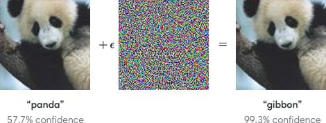
Look at this image below. We have carefully added some carefully selected noise to the image of the panda. After adding the noise, the image still looks like a Panda to a human but the machine learning model gets confused and predicts as gibbon.
Initially, it was argued that Adversarial examples are specific to Deep Learning due to the high amount of non-linearity present in them. While later explanations specify the primary cause of neural networks’ vulnerability to adversarial perturbation is their linear nature. Hence, not only deep learning but a lot of machine learning models are techniques have the problem of Adversarial examples.
Types of Adversarial Attacks
These kinds of attacks pose a serious security risk to machine learning systems like self-driving car, Amazon Go stores, Alexa, Siri etc. If the attacker has the access to the information about the underlying model parameters and architecture, it’s called a White Box Attack which is not very common. On the other hand, if the attacker has no access to the deployed model architecture etc., the attack is called a Black Box Attack. Another worrying observation is that an adversarial example created for one machine learning model is usually misclassified by other models too, even when the other models had different architectures or were trained on a different dataset. Moreover, when these different models misclassify, they make the same prediction. This basically means that the attacker doesn’t need to know the underlying architecture or model parameters. An attacker can just create his/her own model and create an adversarial example for that model. It’s likely that the example created will break most of the other machine learning systems too.
Adversarial attacks that just want your model to be confused and predict a wrong class are called Untargeted Adversarial Attacks. However, the attacks which compel the model to predict a (wrong) desired output are called Targeted Adversarial attacks. Think about it, Targeted Adversarial attacks are very powerful and dangerous. If you can make a driverless car read the red light as green, it would be scary.
So, how are these inputs crafted?
There are several algorithms which can generate adversarial examples effectively for a given model. In this blog post, we will be discussing a few of these methods such as Fast Gradient Sign Method(FGSM) and implementing them using Tensorflow.
1. Fast Gradient Sign Method(FGSM)
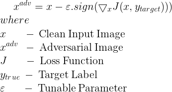
FGSM is a single step attack, ie.. the perturbation is added in a single step instead of adding it over a loop (Iterative attack). The perturbation in FGSM is given by the following equation.
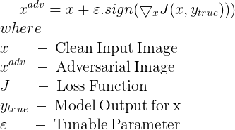
The above equation performs an untargeted attack on the image ie.. the adversarial image generated is not targeted to maximize predictions for a particular class. Gradient can be calculated using back-propagation.
For a targeted FGSM attack, the following equation is used.
What we saw above were single step attacks. However, instead of adding the perturbation in a single step, it can be added over a loop as well. Next, we are going to describe a simple iterative attack method, which will further be used in a highly effective Iterative Least-Likely Class Method.
Here is the Tensorflow code for this method:
|
1 2 3 4 5 6 7 8 9 10 11 |
def step_fgsm(x, eps, logits): label = tf.argmax(logits,1) one_hot_label = tf.one_hot(label, NUM_CLASSES) cross_entropy = tf.losses.softmax_cross_entropy(one_hot_label, logits, label_smoothing=0.1, weights=1.0) x_adv = x + eps*tf.sign(tf.gradients(cross_entropy,x)[0]) x_adv = tf.clip_by_value(x_adv,-1.0,1.0) return tf.stop_gradient(x_adv) |
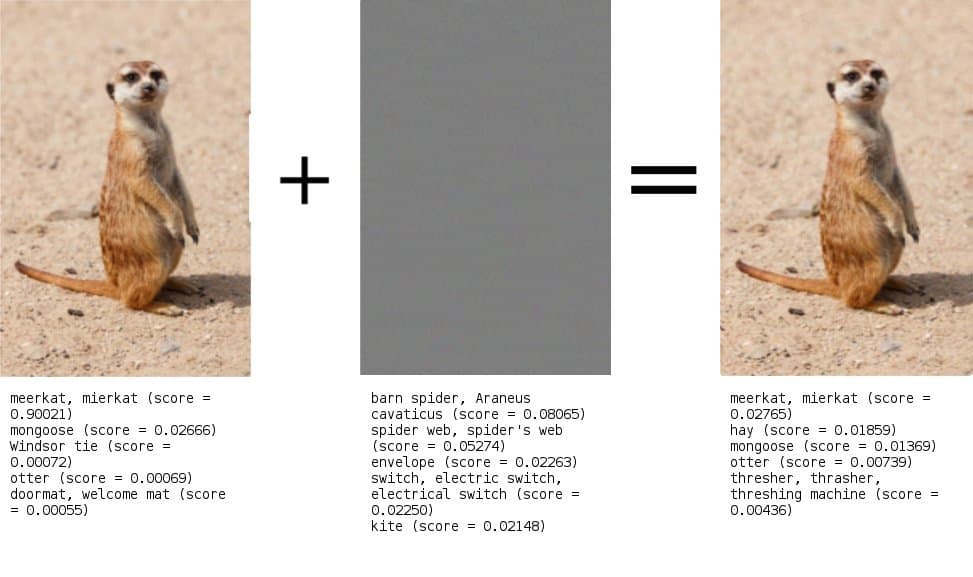
Let’s apply this an image of Meerkat and see if it will confuse InceptionV3 architecture trained on ImageNet dataset. As you can see that it confuses the model but doesn’t break it completely. Meerkat is still the most likely class.
2. Basic Iterative Method
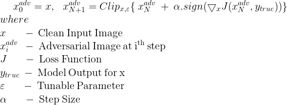
Instead of applying the perturbation in a single step, it is applied multiple times with a small step size. In this method, the pixel values of intermediate results are clipped after each step to ensure that they are in an ? neighbourhood of the original image ie.. within the range [Xi,j−?,Xi,j+?], Xi,j being the pixel value of the previous image.
The equation for generating perturbed images using this method is given by
Let’s write the code to apply this adversarial method:
|
1 2 3 4 5 6 7 8 9 10 11 |
def step_targeted_attack(x, eps, one_hot_target_class, logits): #one_hot_target_class = tf.one_hot(target, NUM_CLASSES) #print(one_hot_target_class,"\n\n") cross_entropy = tf.losses.softmax_cross_entropy(one_hot_target_class, logits, label_smoothing=0.1, weights=1.0) x_adv = x - eps * tf.sign(tf.gradients(cross_entropy, x)[0]) x_adv = tf.clip_by_value(x_adv, -1.0, 1.0) return tf.stop_gradient(x_adv) |
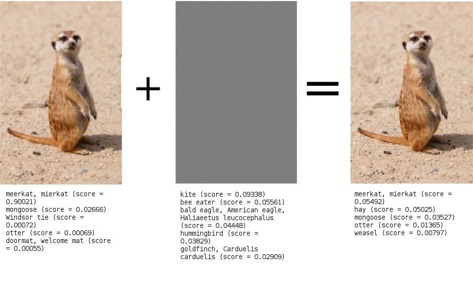
Applying on the same image of Meerkat, we get similar result.
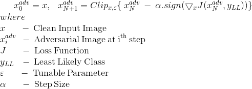
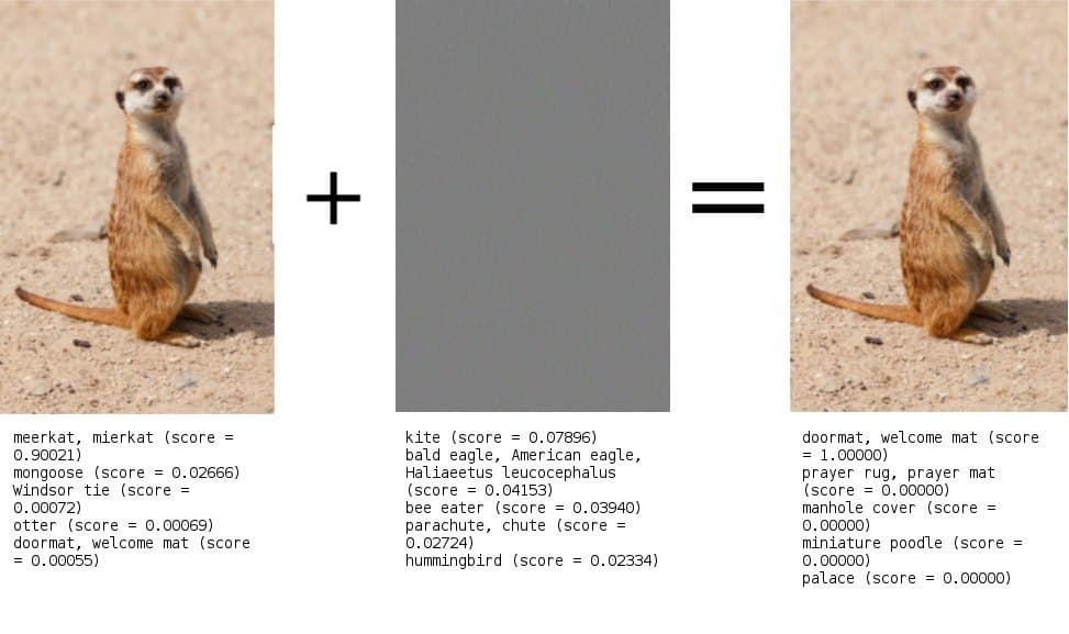
3. Iterative Least-Likely Class Method
This iterative method tries to make an adversarial image which will be classified as the class with the lowest confidence score in the prediction of the clean image.
yLL = argminy{p(y|X)}
For a classifier trained on a large training dataset, the least likely class would be highly dissimilar from the correct one. This leads to more interesting misclassification, like classifying a dog as a car.
To make an adversarial image which is classified as yLL, we need to make a targeted attack using yLL as the target class.
Previously, we didn’t really explain the minus sign with the perturbation in the targeted attack method. In FGSM, to maximize the loss for the correct class, i.e. ytrue , the sign function is applied to the loss function with respect to ytrue and is added to the image. In the same way, in order to minimize the loss for the incorrect class i.e. ytarget, the sign function is applied to the loss function wrt ytarget and is subtracted from the image.
The equation for the same is given by
Let’s code this in Tensorflow to generate our adversarial examples.
|
1 2 3 4 5 6 7 |
def step_ll_adversarial_images(x, eps, logits): least_likely_class = tf.argmin(logits, 1) one_hot_ll_class = tf.one_hot(least_likely_class, NUM_CLASSES) one_hot_ll_class = tf.reshape(one_hot_ll_class,[1,NUM_CLASSES]) # This reuses the method described above return step_targeted_attack(x, eps, one_hot_ll_class,logits) |
This confuses the model completely:
Comparison of Adversarial Attacks:
Now that we have described all these methods to generate adversarial examples, which one should we use?
This comparative analysis, as described in this paper, shows how these methods perform on InceptionV3 evaluated on the 50000 validation images of Image Net varying the ? from 2 to 128.
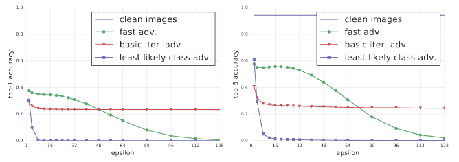
As you can see in the figure above, least likely class method outperforms other methods in terms of the classification accuracy. However, this is an active research area and we keep seeing new methods to generate adversarial examples.
Generating Adversarial examples using Tensorflow(Running the code on InceptionV3):
Here is the code to run inference on the image using these functions. In the Inception model graph, “DecodeJpeg/contents:0” tensor is supposed to hold the raw image (in bytes) while the “Mul:0” tensor is supposed to contain the decoded image after preprocessing.
I have written function calls for various methods in the code, most of them are commented out. You can try all of them with different combinations of ε and iteration count. Although the code describes an iterative attack, you can also try step attacks.
|
1 2 3 4 5 6 7 8 9 10 11 12 13 14 15 16 17 18 19 20 21 22 23 24 25 26 27 28 29 30 31 32 33 34 35 36 37 38 39 40 41 42 43 44 45 46 47 48 49 50 51 52 53 54 55 56 57 58 59 60 61 62 63 64 65 66 67 68 69 70 71 72 73 74 75 76 77 78 79 80 81 82 83 |
def run_inference_on_image(image): """Runs inference on an image. Args: image: Image file name. Returns: Nothing """ if not tf.gfile.Exists(image): tf.logging.fatal('File does not exist %s', image) image_data = tf.gfile.FastGFile(image, 'rb').read() original_shape = cv2.imread(image).shape # Creates graph from saved GraphDef. create_graph() with tf.Session() as sess: # Some useful tensors: # 'softmax:0': A tensor containing the normalized prediction across # 1000 labels. # 'pool_3:0': A tensor containing the next-to-last layer containing 2048 # float description of the image. # 'DecodeJpeg/contents:0': A tensor containing a string providing JPEG # encoding of the image. # Runs the softmax tensor by feeding the image_data as input to the graph. softmax_tensor = sess.graph.get_tensor_by_name('softmax:0') image_tensor = sess.graph.get_tensor_by_name('Mul:0') image = sess.run(image_tensor,{'DecodeJpeg/contents:0': image_data}) predictions = sess.run(softmax_tensor, {'Mul:0': image}) predictions = np.squeeze(predictions) print("Generating Adversial Example...\n\n") target_class = tf.reshape(tf.one_hot(972,NUM_CLASSES),[1,NUM_CLASSES]) adv_image_tensor,noise = step_targeted_attack(image_tensor, 0.007, target_class, softmax_tensor) #adv_image_tensor,noise = step_ll_adversarial_images(image_tensor, 0.007, softmax_tensor) #adv_image_tensor,noise = step_fgsm(image_tensor, 0.007, softmax_tensor) #adv_image = sess.run(adv_image_tensor,{'DecodeJpeg/contents:0': image_data}) adv_image = image adv_noise = np.zeros(image.shape) for i in range(10): print("Iteration "+str(i)) adv_image,a = sess.run((adv_image_tensor,noise),{'Mul:0': adv_image}) adv_noise = adv_noise + a plt.imshow(image[0]/2 + 0.5) #plt.show() save_image(image,original_shape,"original.jpg") plt.imshow(adv_image[0]/2 + 0.5) #plt.show() save_image(adv_image,original_shape,"adv_image.jpg") plt.imshow(adv_noise[0]/2 + 0.5) #plt.show() save_image(adv_noise,original_shape,"adv_noise.jpg") adv_predictions = sess.run(softmax_tensor, {'Mul:0' : adv_image}) adv_predictions = np.squeeze(adv_predictions) noise_predictions = sess.run(softmax_tensor, {'Mul:0' : adv_noise}) noise_predictions = np.squeeze(noise_predictions) # Creates node ID --> English string lookup. node_lookup = NodeLookup() print("\nNormal Image ...\n") top_k = predictions.argsort()[-FLAGS.num_top_predictions:][::-1] for node_id in top_k: human_string = node_lookup.id_to_string(node_id) score = predictions[node_id] print('%s (score = %.5f)' % (human_string, score)) print("\nAdversial Image ...\n") top_k = adv_predictions.argsort()[-FLAGS.num_top_predictions:][::-1] for node_id in top_k: human_string = node_lookup.id_to_string(node_id) score = adv_predictions[node_id] print('%s (score = %.5f)' % (human_string, score)) print("\nAdversial Noise ...\n") top_k = noise_predictions.argsort()[-FLAGS.num_top_predictions:][::-1] for node_id in top_k: human_string = node_lookup.id_to_string(node_id) score = noise_predictions[node_id] print('%s (score = %.5f)' % (human_string, score)) |
In this case, we used 0.07 for ε and 10 as the number of iterations. You can play around with these values and see the results for yourselves. Instead of an iterative method, a step method can also be used.
Safeguarding against Adversarial attacks:
How can we prevent our models from such attacks? One of the most effective technique is to use the adversarial examples for training i.e. we generate a lot of adversarial examples and use them during training so that our network learns to avoid these. Another technique to prevent adversarial attacks is defensive distillation. We will discuss these defense mechanisms in a future post.
The code for this post can be found here.
Appendix:
Here is the list of many popular methods to generate adversarial examples.
- Fast Gradient Sign Method – Goodfellow et al. (2015)
- Basic Iterative Method – Kurakin et al. (2016)
- Jacobian-based Saliency Map Method – Papernot et al. (2016)
- Carlini Wagner L2 – Carlini and Wagner(2016)
- DeepFool – Moosavi-Dezfooli et al. (2015)
- Elastic Net Method – Chen et al. (2017)
- Feature Adversaries – Sabour et al. (2016)
- LBFGS – Szegedy et al. (2013)
- Projected Gradient Descent – Madry et al. (2017)
- The Momentum Iterative Method – Dong et al. (2017)
- SPSA – Uesato et al. (2018)
- Virtual Adversarial Method – Miyato et al. (2016)
- Single Pixel attack.