So you trained a new model using Tensorflow and now you want to show it off to your friends and colleagues on a website for a hackathon or a new startup idea. Let’s see how to achieve that.

A typical Tensorflow model contains 4 files:
|
1 2 3 4 5 6 |
saver = tf.train.import_meta_graph('./dogs-cats-model.meta', clear_devices=True) graph = tf.get_default_graph() input_graph_def = graph.as_graph_def() sess = tf.Session() saver.restore(sess, "./dogs-cats-model") |
|
1 2 3 4 5 6 7 |
output_node_names="y_pred" output_graph_def = graph_util.convert_variables_to_constants( sess, # The session input_graph_def, # input_graph_def is useful for retrieving the nodes output_node_names.split(",") ) |
|
1 2 3 4 5 6 |
output_graph="/dogs-cats-model.pb" with tf.gfile.GFile(output_graph, "wb") as f: f.write(output_graph_def.SerializeToString()) sess.close() |
|
1 2 3 4 5 |
frozen_graph="./dogs-cats-model.pb" with tf.gfile.GFile(frozen_graph, "rb") as f: restored_graph_def = tf.GraphDef() restored_graph_def.ParseFromString(f.read()) |
|
1 2 3 4 5 6 7 8 |
with tf.Graph().as_default() as graph: tf.import_graph_def( restored_graph_def, input_map=None, return_elements=None, name="" ) |
|
1 2 3 4 5 |
a, b= tf.import_graph_def(graph_def, return_elements=['inputs', 'fc8/predictions'], name='') |
|
1 2 3 4 5 6 7 8 9 10 11 12 13 14 15 16 17 18 19 20 21 22 23 24 25 26 27 28 29 30 31 32 33 34 35 36 37 38 39 40 41 42 43 44 45 46 47 48 49 |
import tensorflow as tf import os import numpy as np import os,glob,cv2 import sys,argparse # First, pass the path of the image dir_path = os.path.dirname(os.path.realpath(file)) image_path=sys.argv[1] filename = dir_path +'/' +image_path image_size=128 num_channels=3 images = [] ## Reading the image using OpenCV image = cv2.imread(filename) ## Resizing the image to our desired size and preprocessing will be done exactly as done during training image = cv2.resize(image, (image_size, image_size), cv2.INTER_LINEAR) images.append(image) images = np.array(images, dtype=np.uint8) images = images.astype('float32') images = np.multiply(images, 1.0/255.0) ## The input to the network is of shape [None image_size image_size num_channels]. ## Hence we reshape. x_batch = images.reshape(1, image_size,image_size,num_channels) frozen_graph="./dogs-cats-model.pb" with tf.gfile.GFile(frozen_graph, "rb") as f: graph_def = tf.GraphDef() graph_def.ParseFromString(f.read()) with tf.Graph().as_default() as graph: tf.import_graph_def(graph_def, input_map=None, return_elements=None, name="" ) ## NOW the complete graph with values has been restored y_pred = graph.get_tensor_by_name("y_pred:0") ## Let's feed the images to the input placeholders x= graph.get_tensor_by_name("x:0") y_test_images = np.zeros((1, 2)) sess= tf.Session(graph=graph) ### Creating the feed_dict that is required to be fed to calculate y_pred feed_dict_testing = {x: x_batch} result=sess.run(y_pred, feed_dict=feed_dict_testing) print(result) |
|
1 2 |
pip install flask |
Now, we shall add all the code we discussed above in a webapp.py file after creating a flask app. Let’s first create a flask app:
|
1 2 3 |
import flask app = flask.Flask(__name__) |
The frozen weights are 8 MB in our case. If webserver has to load weights for each request and then do the inference, it will take a lot more time. So, we shall create the graph and load the weights and keep that in the memory so that we can quickly serve each incoming request.
|
1 2 3 4 5 6 7 8 9 10 11 12 13 14 |
def load_graph(trained_model): with tf.gfile.GFile(trained_model, "rb") as f: graph_def = tf.GraphDef() graph_def.ParseFromString(f.read()) with tf.Graph().as_default() as graph: tf.import_graph_def( graph_def, input_map=None, return_elements=None, name="" ) return graph |
And then call this function at the start of the webserver, so that it’s accessible for each request and happens only once.
|
1 2 3 4 |
app.graph=load_graph('./dogs-cats-model.pb') if __name__ == '__main__': app.run(host="0.0.0.0", port=int("5000"), debug=True, use_reloader=False) |
Finally, we create an end-point for our web-server which allows an user to upload an image and run prediction:
|
1 2 3 4 5 6 7 8 9 10 11 12 13 14 15 16 17 18 19 20 21 22 23 24 25 26 27 28 29 30 31 32 33 34 35 36 37 38 39 40 |
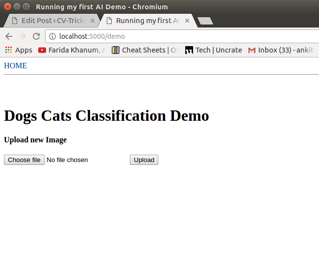
@app.route('/demo',methods=['POST','GET']) def demo(): if request.method == 'POST': //Code for prediction/inference goes here return ''' <!doctype html> <html lang="en"> <head> <title>Running my first AI Demo</title> </head> <body> <div class="site-wrapper"> <div class="cover-container"> <nav id="main"> <a href="http://localhost:5000/demo" >HOME</a> </nav> <div class="inner cover"> </div> <div class="mastfoot"> <hr /> <div class="container"> <div style="margin-top:5%"> <h1 style="color:black">Dogs Cats Classification Demo</h1> <h4 style="color:black">Upload new Image </h4> <form method=post enctype=multipart/form-data> <p><input type=file name=file> <input type=submit style="color:black;" value=Upload> </form> </div> </div> </div> </div> </div> </body> </html> ''' |
Once, done we can upload an image using the UI here:

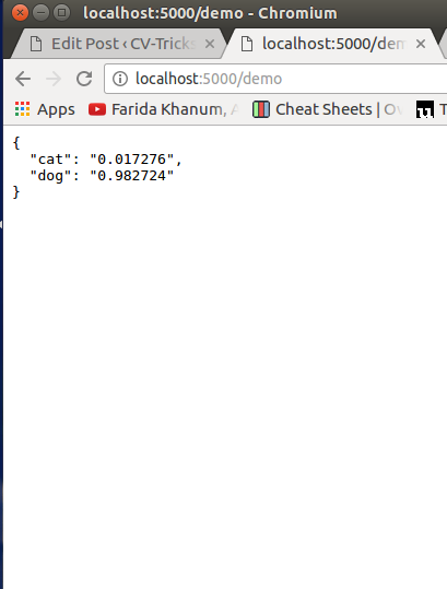
After clicking, upload you can see the results like this:

Hopefully, this post helps you in showing off your newly trained model. May be you could build the hotDog vs not-hotDog model and raise millions of dollars for your cool new startup. However, the way to deploy a tensorflow model on production is Tensorflow-Serving infrastructure which we shall cover in a future post. The code shared in this post can be downloaded from our github repo.


