Artificial Intelligence has improved quite a lot in the last decade. By improvement I mean we’re able to do things better than before as well as we can now do things that we didn’t even imagine, but now we and machines both can imagine. What ! machines can imagine ? Yes you heard it right ! This all goes to Generative Adversarial Networks – a simple deep learning network that can do wonders if properly configured.
Let’s dive deeper to understand Generative Adversarial Network(GAN). GAN is based on three concepts – Generative, Adversarial and Networks. So let’s begin with Network first.
NETWORK :
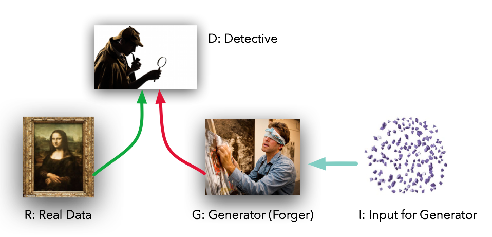
Basically the network here means a multilayer perceptron network, though we use more advanced architecture, but for now let’s keep it simple. So there are two networks, Discriminator and Generator. Consider we’ve a cat image dataset (28*28 images) and a function that generates uniform noise of given shape (let’s say 1*100). So we give this uniform noise to the Generator and it’ll generate a 28*28 image from the noise. Let’s call it fake image (initially it’ll be just random noise). So we’ve real image from the cat dataset and fake image from the Generator, now we’ll challenge the Discriminator to tell which one is real image. You can picture the Discriminator as Detective and Generator as Forger.
Obviously in the start Discriminator will easily distinguish between both, but here is the nice concept. From the response of Discriminator, Generator network will alter its weights.You can think of it like Discriminator is telling you the probability of an image to be a real image. So initially it’ll be around 1 for real image and 0 for fake image. So we’ll take the difference and give it to the Generator, therefore the Generator will know how far it is from generating images like real ones and alter it’s weights accordingly.
ADVERSARIAL :
Here comes the concept of Adversarial. Adversarial basically means a situation involving opposition or conflicts. If you look deeper you’ll see that’s exactly what’s happening. While Discriminator has to differentiate between real and fake image, Generator is trying to Generate images, that is similar to real image so that Discriminator can no more distinguish between then. That is Generator is just trying to fool the Discriminator while the Discriminator is trying not to get fooled (hence conflict).
GENERATIVE :
So once you train the two networks enough that the Discriminator is no more able to distinguish between real and fake image, giving probability of 0.5 for each image(optimal condition), that means Generator is generating as good image as the real one. But since the generated images comes from a random noise (that 1*100), no matter how much similar the image would be from the real one, it’ll be a unique image. Hence essentially the Generator is generating brand new images, and hence the word Generative.
So here is the complete flow of what we’re trying to do :

SIMPLE IMPLEMENTATION :
Now we have basic understanding of GAN let’s quickly code a basic GAN. We’ll use MNIST dataset for this implementation, that is we’ll try to generate new images of the digits in the MNIST dataset.
Let’s start with Discriminator Network. It takes a data sample as input and predicts the probability of it coming from original MNIST dataset. In this case input will be vector of size 784 (MNIST images have resolution 28x28x1) and output will be of size 1(probability). In between we’ll use two fully connected layers that’ll simply downsample the input size. For activation we’ll use rectilinear linear unit for hidden layers and sigmoid activation for the last layer as probability ranges between (0,1).
|
1 2 3 4 5 6 7 8 9 |
def DN(X,reuse=None): with tf.variable_scope('dis',reuse=reuse): layer1 = tf.layers.dense(X,256,activation=tf.nn.relu) layer2 = tf.layers.dense(layer1,128,activation=tf.nn.relu) output = tf.layers.dense(layer2,1,activation=tf.nn.sigmoid) return output |
Next we’ll define the Generator Network. It takes a noise vector of size 100 and outputs a fake image of size 784 (same as MNIST samples). In between we’ll use two fully connected layers that’ll upsample the noise. Here also we’ll use rectilinear linear unit for activation in the hidden layers, but for the last layer we’ll use hyperbolic tangent activation as in MNIST dataset pixel values are normalised between (-1,1).
|
1 2 3 4 5 6 7 8 9 |
def GN(z,reuse=None): with tf.variable_scope('gen',reuse=reuse): layer1 = tf.layers.dense(z,256,activation=tf.nn.relu) layer2 = tf.layers.dense(layer1,512,activation=tf.nn.relu) output = tf.layers.dense(layer2,784,activation=tf.nn.tanh) return output |
Now we have the networks let’s take their outputs. First we’ll give noise to Generator which in return will generate a fake image. Then we take this fake image and a sample from original dataset and input both of them one by one to Discriminator Network. For we’ll first define placeholders for image sample and noise :
|
1 2 3 |
real_image = tf.placeholder(tf.float32,shape=(None,784)) z = tf.placeholder(tf.float32,shape=(None,100)) |
Now we’ll take the outputs from the two network :
|
1 2 3 4 |
fake_image = GN(z) real_logit = DN(real_image) fake_logit = DN(fake_image, reuse=True) |
If you visualise the image Generated by Generator network initially it’ll be noise only. So we need to tell the Generator that it is performing very bad and it need to alter its weights in order to generate better quality image. For this we’ll define loss functions for both the network that’ll essentially indicate how bad they’re performing.
So how do we define loss functions for simple classification problem (like cat and dog classification). We give the image as input to our model and tell it to predict one of two classes. Then we take the prediction and compare with original labels and take root mean square difference as the loss. So far good. We can define the loss function for Discriminator in the same way. We input a sample to the network, then it predicts the probability that we’ll compare with its label (let’s sat 1 for real image and 0 for fake image). But what for Generator Network ? Generator is generating brand new images, duly there are no labels for that images to compare with. So how do we define the loss for generator network which is working in unsupervised manner.
So there is small trick to define the losses which actually originates from the minimax game theory. There is a concept of value function in game theory. Consider a football game between team A and B. A’s value function is to maximise goal count of A and minimise goal count of B, while B is doing the reverse, maximising goal count of B and minimising goal count of A. In game theory, we call this type of game as min-max game (assuming each team as one player), because one player is trying to maximise the same value function which other is minimising
If you look closely at the fundamental working of Generator and Discriminator network, you can infer basically they’re playing a mini-max game. Generator wants the Discriminator to classify fake image as real while the Discriminator wants the opposite. So we can define a value function which one of them will maximise while another will minimise.
|
1 2 3 |
d_value = tf.reduce_mean(tf.log(real_logit) + tf.log(1. - fake_logit )) g_value = -tf.reduce_mean(tf.log(real_logit) + tf.log(1. - fake_logit )) |
Where d_value is Discriminator value function and g_value is Generator value function. Discriminator is maximising the probability of it predicting the real image as 1 and fake image as 0 while Generator is minimising the same. Note we used negative sign in the Generator Value function since it is minimising it.
Now the real_logit is independent of Generator network, so we can remove it from the Generator value function. Also instead of Generator minimising probability of Discriminator classifying the fake image as 0, we can change it such that it’ll maximise the probability of Discriminator classifying fake image as 1. This results in stable gradient initially. So here are the changed value functions :
|
1 2 3 |
d_value = tf.reduce_mean(tf.log(real_logit) + tf.log(1. - fake_logit )) g_value = tf.reduce_mean(tf.log(fake_logit)) |
Since in Tensorflow we can only minimise value, we’ll take negative of the value functions to define our loss function :
|
1 2 3 |
d_loss = - tf.reduce_mean(tf.log(real_logit) + tf.log(1. - fake_logit )) g_loss = - tf.reduce_mean(tf.log(fake_logit)) |
So now we have the loss functions, we need to define the optimisers to alter the network weights according the Gradient Descent rule. Before that we’ll take the Discriminator and Generator variables separately.
|
1 2 3 4 |
allvars = tf.trainable_variables() dvars = [var for var in allvars if 'dis' in var.name] gvars = [var for var in allvars if 'gen' in var.name] |
Now we’ll define separate optimisers for Discriminator and Generator network. We’ll use Adam Optimiser as it performs well in most of the cases with learning rate 0.0001
|
1 2 3 |
doptimizer = tf.train.AdamOptimizer(learning_rate=0.0001).minimize(d_loss,var_list=dvars) goptimizer = tf.train.AdamOptimizer(learning_rate=0.0001).minimize(g_loss,var_list=gvars) |
Let’s just quickly summarise what have we done till now – we defined the Generator and Discriminator network. loss functions for the two network and separate optimisers for both the them. So what left ! Hard part is done now we just need to take out the data and train the model.
One thing to note here. We’ve two networks to train simultaneously. Let’s see what are the difference way we can train both :
- Train Discriminator more than Generator : Generator varies it’s weights according to the response from Discriminator (remember real_image – fake_image). So if the Discriminator starts playing very optimally in the beginning, the gradients if the Generator will be close to zero and the network will suffer vanishing gradient problem.
- Train Generator more that Discriminator : If we train Discriminator less than the Generator, Generator will not get accurate response from the Discriminator, and it’ll never be able to generate good quality data.
- Train them alternately : That seems the best idea. In this way neither Discriminator will oppress the Generator, nor it’ll give vague response to the Generator.
|
1 2 3 4 5 |
with tf.Session()) as sess: sess.run(tf.global_variables_initializer()) for epoch in range(epoch): for i in range(mnist.train.num_examples//batch_size): |
Take a batch of data from MNIST dataset :
|
1 2 3 |
batch_data = mnist.train.next_batch(batch_size=batch_size) ximage = batch_data[0].reshape((batch_size,784)) |
Sample a noise from uniform distribution :
|
1 2 |
xsample = np.random.uniform(-1.,1.,size=(batch_size,100)) |
Now run both the optimisers :
|
1 2 3 |
sess.run(doptimizer,feed_dict={real_image:ximage,z:xsample}) sess.run(goptimizer,feed_dict={z:xsample}) |
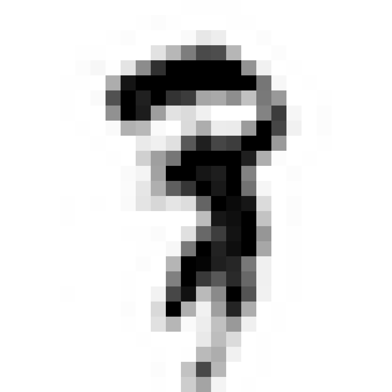
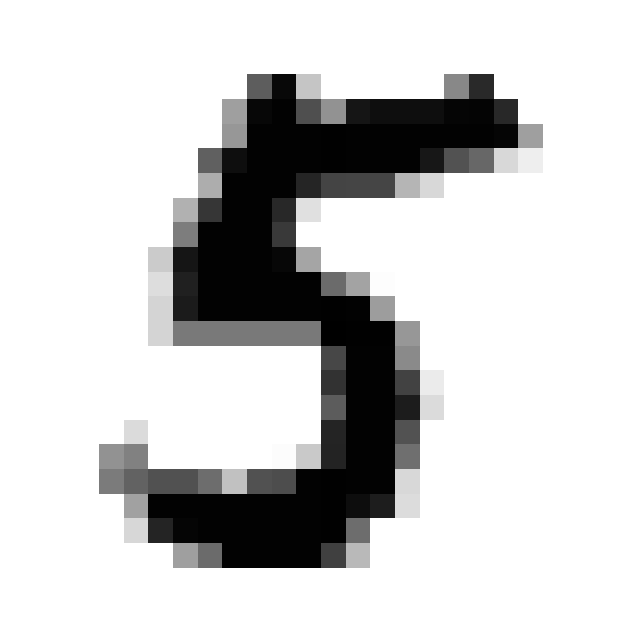
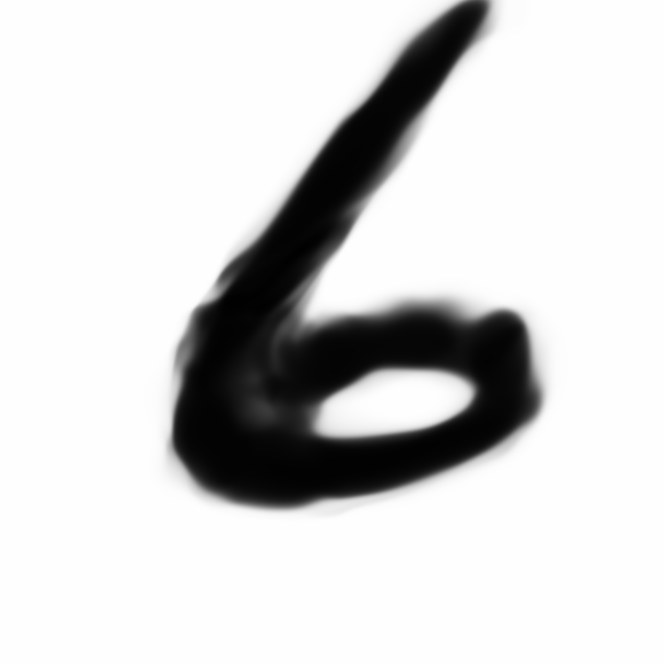
And that’s it. Train this model for 1000 epoch, take image samples at each 10 epochs and you’ll see how quickly the Generator makes improvement and generates similar images to real one. I’ve attached some images from my model. First image is after 2 epochs while last one is after 400 epochs.