Keras is winning the world of deep learning. In this tutorial, we shall learn how to use Keras and transfer learning to produce state-of-the-art results using very small datasets. We shall provide complete training and prediction code. For this comprehensive guide, we shall be using VGG network but the techniques learned here can be used to finetune Alexnet, Inception, Resnet or any other custom network architecture. In a previous tutorial, we used 2000 images of dog and cat to get a classification accuracy of 80%. However, with transfer learning, we shall achieve 98% accuracy with just 500 images each of dog and cat class.
Why do Neural Networks need huge data?
Deep Learning is the new state-of-the-art. But it needs huge amount of training data. Why is that? Multilayer Feedforward networks are universal Approximator i.e. multilayer feed-forward neural networks can be used to model any problem. So, there are no theoretical constraints for their success. However, in the real world, there are so many constraints like insufficient data, limited compute etc. Fortunately, some of the network architectures(like alexnet, Vgg, Inception, Resnet etc) have been found to be great at the task of learning and they have been openly shared by the vibrant computer vision community. However, most of these networks have millions of parameters. If we train these networks with small datasets then it will result in overfitting meaning the network will only work for examples in training data or exactly similar examples but will not generalize well(will not work on additional examples).
Learning with little data(Transfer learning aka Fine-tuning):
In practice, instead of training our networks from scratch, everyone just first trains the network on 1.2 million images belonging to 1000 different classes from Imagenet data-set. These weights are saved and such saved weights are called ImageNet Pretrained weights. When one starts working on a specific problem where a small amount of training data is available, one takes these pre-trained weights and continue training. One should keep this in mind that the images for the task must be similar to ImageNet dataset otherwise the previously learning will not be that useful. For example if we have to do some training on medical images like MRI and X-Ray images then ImageNet pretrained models will not be of great use. Here is a loose analogy to transfer learning: Kids learn to read by alphabets and eventually when they are familiar with the language, they start reading by words. Pretraining our networks on ImageNet selects our weights in such a way that network becomes familiar with the kind of images that are common in our world. When we train these with small data during transfer learning, it’s easier to reach the weights that solve our problem.
Strategies for Fine tuning:
-
Linear SVM on top of bottleneck features
If you have very little data, it won’t be possible to do much training. The best strategy for this case will be to train an SVM on top of the output of the convolutional layers just before the fully connected layers( also called bottleneck features).
-
Just Replace and train the last layer
ImageNet pretrained models will have 1000 outputs from last layer, you can replace this our own softmax layers, for example in order to build 5 class classifier our softmax layer will have 5 output classes. Now, the back-propagation is run to train the new weights. In this case, however, it’s likely for us to overfit so a lot of data augmentation and proper cross-validation is important.
-
Train only last few layers
Depending on the amount of data available to you, the complexity of the problem you are solving, one can choose to freeze(don’t change weights during backpropagation) first few layers and train only last few layers. The initial layers of convolutional neural networks just learn the general features like edges and very general image features, it’s the deeper part of the networks that learn the specific shapes and parts of objects which are trained in this method. Another similar method is to use 0 or very small learning rate during the initial layers and using higher learning rate for the layers that are deeper.
-
Freeze, Pre-train and Finetune(FPT)
It’s one of the most effective technique in my experience and this is exactly what I will demonstrate in the code below. There are two steps involved here: a) Freeze and Pretrain: First replace the last layer with a small mini network of 2 small Fully connected layers. Now, freeze all the pretrained layers and train the new network. Save the weights of this network(let’s call them pretrained weights) b) Finetune: Load the pretrained weights and train the complete network with a smaller learning rate. This results in very good accuracy with even small datasets.
-
Train all the layers:
In case you are fortunate to have millions of examples for your training, you can start with pretrained weights but train the complete network.
In the following section, we shall use fine tuning on VGG16 network architecture to solve a dog vs cat classification problem.
Finetuning VGG16 using Keras:
VGG was proposed by a reasearch group at Oxford in 2014. This network was once very popular due to its simplicity and some nice properties like it worked well on both image classification as well as detection tasks. VGG network has many variants but we shall be using VGG-16 which is made up of 5 convolutional blocks and 2 fully connected layers after that. See below:
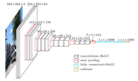
Vgg 16 architecture
Input to the network is 224 *224 and network is:
- Conv Block-1: Two conv layers with 64 filters each. output shape: 224 x 224 x 64
- Max Pool-1: Max-pooling layer that outputs: 112 x 112 x 64
- Conv Block-2: Two conv layers with 128 filters each. output shape: 112 x 112 x 128
- Max Pool-2: Max-pooling layer that outputs: 64 x 64 x 128
- Conv Block-3: Three conv layers with 256 filters each. output shape: 56 x 56 x 256
- Max Pool-3: Max-pooling layer that outputs: 28 x 28 x 256
- Conv Block-4: Three conv layers with 512 filters each. output shape: 28 x 28 x 512
- Max Pool-4: Max-pooling layer that outputs: 14 x 14 x 512
- Conv Block-5: Three conv layers with 512 filters each. output shape: 14 x 14 x 512
- Max Pool-5: Max-pooling layer that outputs: 7 x 7 x 512
- Fc1(fully connected layer 1):output shape: 1x 1 x 4096
- Fc2(fully connected layer 2):output shape: 1x 1 x 4096
- Output(predictions):output shape: 1x1x1000 (For ImageNet)
There are two steps to our training methodology Freeze, Pre-train and Finetune(FPT):
Step-1: Freeze and Pre-train
Step-2: Finetune the pretrained weights.
Let’s go through them one by one.
Step-1: Freeze and Pre-train
Here are the 5 steps that we shall do to perform pre-training:
1. Gather Training and testing dataset:
We shall use 1000 images of each cat and dog that are included with this repository for training. We shall show how we are able to achieve more than 90% accuracy with little training data during pretraining. Here we are preparing to receive path of training and testing data, number of classes via command line arguments.
|
1 2 3 4 5 6 |
img_size=224 ap = argparse.ArgumentParser() ap.add_argument("-train","--train_dir",type=str, required=True,help="(required) the train data directory") ap.add_argument("-num_class","--class",type=int, required=True,help="(required) number of classes to be trained") ap.add_argument("-val","--val_dir",type=str, required=True,help="(required) the validation data directory") |
2. Image Augmentation:
It’s a standard practice in computer vision to augment the training dataset and prepare many examples from whatever data we have. Some of the common augmentations are like slight rotations, flipping images, small random crops etc. Idea is to add small perturbations without damaging the central object so that neural network is more robust to these kinds of real-world variations. Fortunately, keras provides a mechanism to perform these kinds of data augmentations quickly. ImageDataGenerator is an in-built keras mechanism that uses python generators ensuring that we don’t load the complete dataset in memory, rather it accesses the training/testing images only when it needs them. Another important thing to note here is we normalize by dividing each pixel value in all the images by 255, since we are using 8bit images so each pixel value is now between 0 and 1. This is also loosely called pre-processing of input images for VGG network. Our imagenet weights have also been obtained using the same normalization. Hence, if you miss this, you will get very bad predictions.
|
1 2 3 4 5 6 7 8 9 10 11 12 13 14 15 16 17 18 19 20 21 |
batch_size=10 train_datagen = image.ImageDataGenerator( rescale=1./255, shear_range=0.2, zoom_range=0.2, horizontal_flip=True) test_datagen = image.ImageDataGenerator(rescale=1. / 255) train_generator = train_datagen.flow_from_directory( args["train_dir"], target_size=(img_size, img_size), batch_size=batch_size, class_mode='categorical') validation_generator = test_datagen.flow_from_directory( args["val_dir"], target_size=(img_size,img_size), batch_size=batch_size, class_mode='categorical') |
3. Network graph and pre-trained weights:
We have already described the architecture above. Since, keras has provided a VGG16 implementation, we shall reuse that. This code is in VGG16.py file in the network folder. If we specify include_top as True, then we will have the exact same implementation as that of Imagenet pretraining with 1000 output classes. But since we only want to classify between dog and cat, we shall take only the initial 5 convolutional blocks.
|
1 2 3 4 5 6 7 8 9 10 11 12 13 14 15 16 17 18 19 20 21 22 23 24 25 26 27 28 29 30 31 32 33 34 35 36 37 38 39 40 |
# Block 1 x = Conv2D(64, (3, 3), activation='relu', padding='same', name='block1_conv1')(img_input) x = Conv2D(64, (3, 3), activation='relu', padding='same', name='block1_conv2')(x) x = MaxPooling2D((2, 2), strides=(2, 2), name='block1_pool')(x) # Block 2 x = Conv2D(128, (3, 3), activation='relu', padding='same', name='block2_conv1')(x) x = Conv2D(128, (3, 3), activation='relu', padding='same', name='block2_conv2')(x) x = MaxPooling2D((2, 2), strides=(2, 2), name='block2_pool')(x) # Block 3 x = Conv2D(256, (3, 3), activation='relu', padding='same', name='block3_conv1')(x) x = Conv2D(256, (3, 3), activation='relu', padding='same', name='block3_conv2')(x) x = Conv2D(256, (3, 3), activation='relu', padding='same', name='block3_conv3')(x) x = MaxPooling2D((2, 2), strides=(2, 2), name='block3_pool')(x) # Block 4 x = Conv2D(512, (3, 3), activation='relu', padding='same', name='block4_conv1')(x) x = Conv2D(512, (3, 3), activation='relu', padding='same', name='block4_conv2')(x) x = Conv2D(512, (3, 3), activation='relu', padding='same', name='block4_conv3')(x) x = MaxPooling2D((2, 2), strides=(2, 2), name='block4_pool')(x) # Block 5 x = Conv2D(512, (3, 3), activation='relu', padding='same', name='block5_conv1')(x) x = Conv2D(512, (3, 3), activation='relu', padding='same', name='block5_conv2')(x) x = Conv2D(512, (3, 3), activation='relu', padding='same', name='block5_conv3')(x) x = MaxPooling2D((2, 2), strides=(2, 2), name='block5_pool')(x) if include_top: # Classification block x = Flatten(name='flatten')(x) x = Dense(4096, activation='relu', name='fc1')(x) x = Dense(4096, activation='relu', name='fc2')(x) x = Dense(classes, activation='softmax', name='predictions')(x) else: if pooling == 'avg': x = GlobalAveragePooling2D()(x) elif pooling == 'max': x = GlobalMaxPooling2D()(x) |
Fine-tuning is one of the most common way to solve problems using AI and Deep learning. That’s why Keras provides us weights without the top along with complete imagenet weights.
|
1 2 3 4 5 6 7 8 9 10 11 12 13 |
if weights == 'imagenet': if include_top: weights_path = get_file('vgg16_weights_tf_dim_ordering_tf_kernels.h5', WEIGHTS_PATH, cache_subdir='models', file_hash='64373286793e3c8b2b4e3219cbf3544b') else: weights_path = get_file('vgg16_weights_tf_dim_ordering_tf_kernels_notop.h5', WEIGHTS_PATH_NO_TOP, cache_subdir='models', file_hash='6d6bbae143d832006294945121d1f1fc') model.load_weights(weights_path) |
This is how we call the above code for VGG16 model.
|
1 2 |
base_model = VGG16.VGG16(include_top=False, weights='imagenet') |
4. Append our network and choose fine-tuning parameters:
Okay, we have created the graph for convolutional blocks of VGG16 network loaded with imagenet pretrained weights. Pay attention here, for fine-tuning during this experiment, we say that we are happy with the weights of these layers so, don’t change these weights, rather we shall change the weights of the small network that we will be added in the next step.
|
1 2 3 4 5 6 |
i=0 for layer in base_model.layers: layer.trainable = False i = i+1 print(i,layer.name) |
Now, we add a mini network on top of that with two final outputs representing probabilities for cat and dog.
|
1 2 3 4 5 6 |
x = base_model.output x = Dense(128, activation='sigmoid')(x) x = GlobalAveragePooling2D()(x) x = Dropout(0.2)(x) predictions = Dense(args["class"], activation='softmax')(x) |
Now, we are ready for pre-training. In the next step, we shall specify the optimizer, loss etc and start the training.
5. Specify the optimizer, loss etc and start the training.
We shall be using Tensorboard which is a very powerful visualization tool used to observe training process of neural networks. You can install it using this command:
|
1 2 |
pip install tensorboard |
What Tensorboard does is that it provides us an option to write the value of any variable used during training to a directory called logdir. These written values can be read and shown in your browser via a webserver that Tensorboard runs. So, when we create a Tensorboard instance we specify the location of this logdir on your computer.
|
1 2 |
tensorboard = TensorBoard(log_dir="logs/{}".format(time())) |
This will create a log folder and save all the Tensorboard data there. During/After the training, we can start the tensorboard server by running this command. This will start a webserver on your local at port 6006.
|
1 2 |
tensorboard --logdir=logs ## Speficy the path which you want to read |
Now, you can visualize the training process in your browser by opening http://localhost:6006.
We shall use Tensorboard via Keras callback utility which is a nice Keras inbuilt utility to run a specific function to during specific times during training like beginning or end of epochs.
We shall also use the callback utility to specify the path and name of the trained model.
|
1 2 3 4 |
filepath = 'cv-tricks_fine_tuned_model.h5' checkpoint = ModelCheckpoint(filepath, monitor='val_loss', verbose=1,save_best_only=True,save_weights_only=False, mode='auto',period=1) callbacks_list = [checkpoint,tensorboard] |
|
1 2 3 4 5 6 7 8 9 10 11 12 13 |
model = Model(inputs=base_model.input, outputs=predictions) model.compile(loss="categorical_crossentropy", optimizer=optimizers.SGD(lr=0.001, momentum=0.9),metrics=["accuracy"]) model.fit_generator( train_generator, steps_per_epoch=100, epochs=10, callbacks = callbacks_list, validation_data = validation_generator, validation_steps=20 ) |
Now, we can start the traing by running our pretraining script with appropriate paths.
|
1 2 |
python 1_vgg16_pretrain.py -train ../tutorial-2-image-classifier/training_data/ -val ../tutorial-2-image-classifier/testing_data/ -num_class 2 |
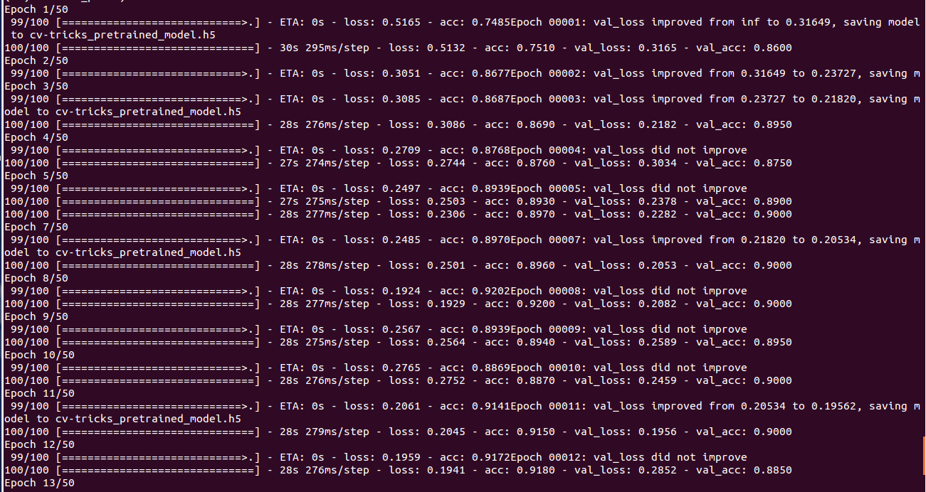
Our training will now start and after pretraining we shall achieve close to 90% with only 500 examples of each class which is impressive considering that in a previous tutorial we were able to achieve only 80% accuracy with more than 2000 examples of each class.
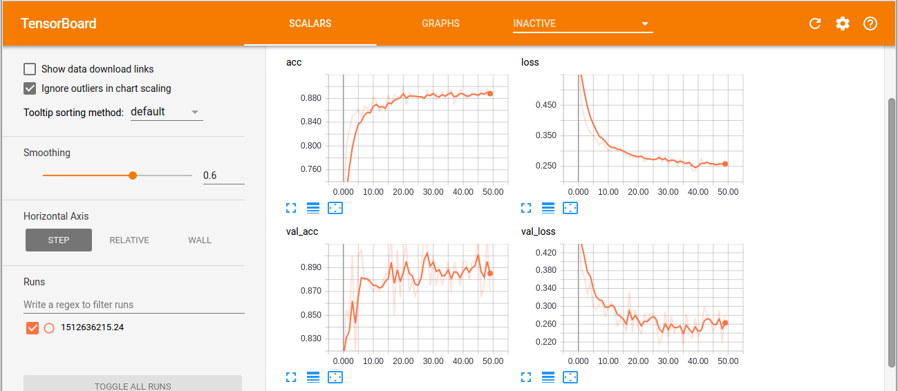
You can see the training and validation accuracy graphs using Tensorboard. Run the graph using:
|
1 2 |
tensorboard --logdir=logs |
Browser on http://localhost:6000/ shows:
Step-2: Finetuning:
In the finetuning step, we shall load the weights(cv-tricks_pretrained_model.h5) saved in pretraining phase. The network will remain the same but we shall not freeze any layers i.e. the weights of all the layers will change during training.
Another important thing to note here is that we will not be loading Imagenet pretrained weights.
|
1 2 3 |
# We pass weights=None since we don't want any weights here base_model = VGG16.VGG16(include_top=False, weights=None) |
Rather, this is how we load the our own pretrained weights:
|
1 2 3 |
# After creating the network model.load_weights("cv-tricks_pretrained_model.h5") |
Important Note:
During Finetuning, we already have a model which is very good so we don’t want to change the weights too much. So, we would use an optimizer with a very slow learning rate. In general, SGD is good choice for this as opposed to adaptive methods like Adam etc.
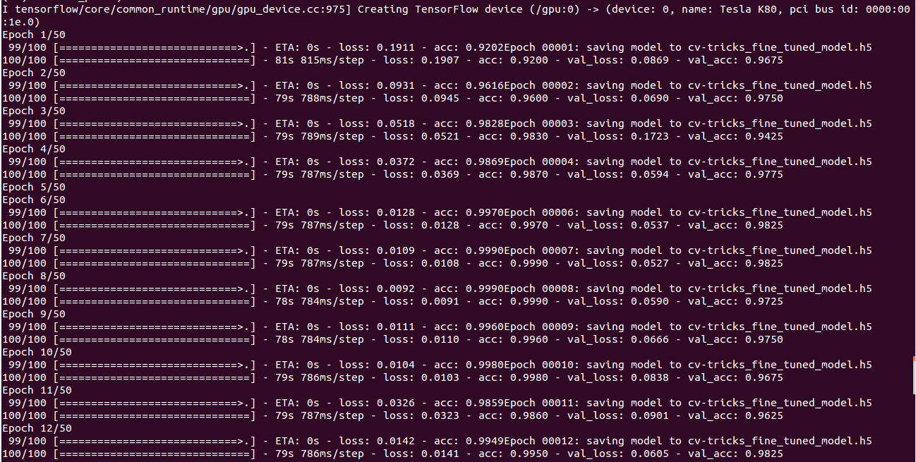
I observed slight overfitting during training so, I increased the dropout to 0.3. Finally, I run the fine-tuning script to start the finetuning process, which gives us a nice cool 98% accuracy with just 500 images of each class.
Prediction:
Now, let’s run this script on a new image to see if our newly trained model able to identify cats and dogs. We shall build the same network graph and load weights that we have trained(cv-tricks_fine_tuned_model.h5). We shall use numpy to load our image and run prediction on it.
|
1 2 3 4 5 6 7 8 9 10 11 12 13 14 15 16 17 18 19 20 |
base_model = VGG16.VGG16(include_top=False, weights=None) x = base_model.output x = Dense(128)(x) x = GlobalAveragePooling2D()(x) predictions = Dense(args["class"], activation='softmax')(x) model = Model(inputs=base_model.input, outputs=predictions) model.load_weights("cv-tricks_fine_tuned_model.h5") inputShape = (224,224) # Assumes 3 channel image image = load_img(args["image"], target_size=inputShape) image = img_to_array(image) # shape is (224,224,3) image = np.expand_dims(image, axis=0) # Now shape is (1,224,224,3) image = image/255.0 preds = model.predict(image) print(preds) |
This prints a list which contains the probabilities for the image containing cat or dog.
|
1 2 |
python 3_predict.py --image test.jpg |
[[ 2.86891848e-13 1.00000000e+00]]
This implies that the image contains a dog and the model very confident about it. Complete code with data can be found here.
And that’s how it’s done. Congratulations! you have learned a very important lesson in your journey to learn AI. It would be a nice idea to try to pick-up a new dataset and train your own classifiers. Or even better use a different network like InceptionV3(which is one of my favorite due to high accuracy/computation ratio). Feel free to share your experience in comments.