In today’s post, we would learn how to identify not safe for work images using Deep Learning.
Not-Safe-For-Work images can be described as any images which can be deemed inappropriate in a workplace primarily because it may contain:
- Sexual or pornographic images
- Violence
- Extreme graphics like gore or abusive
- Suggestive content
For example, LinkedIn is a professional platform where users interact in a professional way. However, it allows users to write and share content. So, it has to ensure that the content is safe for work. Millions of images are uploaded on Linkedin every day, therefore, verifying each and every image manually is an almost impossible task. However, There is an AI for that. In today’s post, we shall learn how any user-generated content platform can fight unwanted content using deep learning and computer vision. We also shall share the code to run a model which has been trained to identify not safe for work images.
Similarly, Most of the other content platforms like YouTube/Instagram where anyone can upload images or videos struggle to keep the platform safe, especially for kids.
Challenges:
Defining NSFW material is subjective and the task of identifying these images is non-trivial. What may be offensive to one person can be loved by another as artistic and acceptable. Or something that is offensive in one context can be acceptable in another. The model shared in today’s post is trained only with pornographic content. The identification of NSFW sketches, cartoons, text, images of graphic violence, or other types of unsuitable content is not addressed with this model. However, you can use the same model to train with other kinds of content as well.
Approach:
We shall use Keras to build an image classifier which separates the images into two types:
- Safe for work
- Not safe for work
In order to build the classifier, we shall use Resnet-50 architecture. Let’s look at the ResNet architectures.

ResNet-50 is computationally expensive. However, we would make some small changes to optimize the architecture a little bit more so that we can easily run this on a CPU machine. We basically reduce the number of filters to half which reduces the number of parameters and computation significantly and we call this network architecture as ResNet50-thin.
Now, this network is trained on Yahoo NSFW dataset which is not released due to the nature of images. However, the model has been released which is shared along with the code of this blog-post.
Identifying NSFW images:
1. Loading pre-trained model:
The original model is trained in Caffe and then converted into Numpy format which can be imported into Tensorflow using Caffe-TensorFlow library. The weight file is called open_nsfw-weights.npy and we can load this into memory using the Numpy load method.
|
1 2 |
self.weights = np.load(weights_path, encoding="latin1").item() |
2. Loading Images and Pre-processing:
The number one mistakes the beginners make while working with deep learning models is in image pre-processing. The most common image format is 8-bit RGB format which encodes each pixel into three channels of Red, Green, Blue each having a value between 0 and 255. In order to handle the variation of intensity and brightness of images, we normalize these values between a small range and then train neural networks. Here are the two most popular normalization methods:
- Mean subtraction: In this case, we can calculate the average value of Red, Green, and Blue channel values of all the images in the whole dataset. This is called the mean value, for example, for ImageNet, this value is R=103.93, G=116.77, and B=123.68. Now, we subtract the mean value from each pixel of the image.
- Divide by maximum value: In this method, we just divide the value of each pixel by 255. This would restrict the value of each channel between 0 and 1. Similarly, some people can choose to restrict the value between -1 to 1 or some similar range. However, we would have to do the same pre-processing during training and deployment.
Let me repeat that. Whatever pre-processing, we do to our images during training must be done exactly the same during inference. In our case, we use mean subtraction:
Code Description
|
1 2 3 4 5 6 7 8 9 10 11 12 13 14 15 16 17 18 19 20 21 22 23 24 25 26 27 28 29 30 31 32 33 34 35 36 37 38 39 40 41 42 43 44 45 46 47 48 49 50 51 52 53 54 55 56 57 58 59 60 61 62 63 64 65 66 67 68 69 70 71 |
# Defining the Mean Subtraction values VGG_MEAN = [104, 117, 123] def create_yahoo_image_loader(expand_dims=True): # Importing the libraries import numpy as np import skimage import skimage.io from PIL import Image from io import BytesIO # Define a new function to load the image def load_image(image_path): # Open the Image file in Read Binary mode pimg = open(image_path, 'rb').read() # Copying the pimg variable to a new variable i.e. img_data img_data = pimg # Creating the buffer for img_data variable and finally opening the image in PIL format from the # new created buffer im = Image.open(BytesIO(img_data)) # Check the mode of the opened image. If the mode is not 'RGB' then convert the image into 'RGB' mode if im.mode != "RGB": im = im.convert('RGB') # Resizing the image into 256x256 imr = im.resize((256, 256), resample=Image.BILINEAR) # Create a new buffer object fh_im = BytesIO() # Saving the resized image into the newly created buffer imr.save(fh_im, format='JPEG') # Setting the pointer fh_im to the start of the buffer fh_im.seek(0) # Open the image using skimage library in the numpy format image = (skimage.img_as_float(skimage.io.imread(fh_im, as_grey=False)) .astype(np.float32)) # Extract the Height, Width and Channels of the image H, W, _ = image.shape # Defining two new variables 'h' and 'w' h, w = (224, 224) # Calculating the offset value for height and width h_off = max((H - h) // 2, 0) w_off = max((W - w) // 2, 0) # Cropping the 224x224 patch from 256x256 image using the calculated offset values image = image[h_off:h_off + h, w_off:w_off + w, :] # RGB to BGR image = image[:, :, :: -1] # Converting the datatype of image to float image = image.astype(np.float32, copy=False) image = image * 255.0 # Applying Mean Subtraction to all the channels image -= np.array(VGG_MEAN, dtype=np.float32) # Expanding the dimension along zeroth axis if expand_dims is set as True if expand_dims: image = np.expand_dims(image, axis=0) return image return load_image |
3. Implementation of Model in TensorFlow
Before building the architecture of the network, let us look into the code where we will build the ResNet-50 blocks.
A) Getting the weights and biases:
The function which is used to get the value of weights and biases is shown below:
|
1 2 3 4 5 6 7 8 9 10 11 12 |
def __get_weights(self, layer_name, field_name): if not layer_name in self.weights: raise ValueError("No weights for layer named '{}' found" .format(layer_name)) w = self.weights[layer_name] if not field_name in w: raise (ValueError("No entry for field '{}' in layer named '{}'" .format(field_name, layer_name))) return w[field_name] |
Parameter Description:
- self: Referring to the calling object
- layer_name: Referring to the layer under question
- field_name: Referring to either weights or biases for the layer under question
Code Description:
Line 3 checks whether the layer_name is present in the weights variable of the object. If the name is not present then an exception will be generated with a message saying that ‘No weights for layer name {layer_name} found’.
If the layer exists then in Line 7 a new variable w is created which has value for the layer under question.
Line 8 checks whether the field_name (weights and biases) are present in the newly created variable i.e. ‘w’. If the field is not present for the layer under question then an exception will be generated with an appropriate message.
Line 9 will return the desired value for the layer under question.
B) Creating a Convolution Layer:
The code for building a convolution layer is shown below:
|
1 2 3 4 5 6 7 8 9 10 11 12 13 14 15 16 17 18 19 20 21 22 23 24 25 26 27 28 29 |
def __conv2d(self, name, inputs, filter_depth, kernel_size, stride=1, padding="same", trainable=False): if padding.lower() == 'same' and kernel_size > 1: if kernel_size > 1: oh = inputs.get_shape().as_list()[1] h = inputs.get_shape().as_list()[1] p = int(math.floor(((oh - 1) * stride + kernel_size - h)//2)) inputs = tf.pad(inputs, [[0, 0], [p, p], [p, p], [0, 0]], 'CONSTANT') else: raise Exception('unsupported kernel size for padding: "{}"' .format(kernel_size)) return tf.keras.layers.Conv2D(filters = filter_depth, kernel_size=(kernel_size, kernel_size), strides=(stride, stride), padding='valid', activation=None, trainable=trainable, name=name, kernel_initializer=tf.constant_initializer( self.__get_weights(name, "weights"), dtype=tf.float32), bias_initializer=tf.constant_initializer( self.__get_weights(name, "biases"), dtype=tf.float32))(inputs) |
Parameter Description:
- self: Referring to the calling object
- name: Layer Name used to identify the layer in the network.
- inputs: Input to the convolution layer
- filter_depth: Number of filters used to do the convolution operation
- kernel_size: Size of each filters
- stride = 1: The amount through which the convolution window should be displaced during the convolution operation. The default value is set to 1.
- padding = “same”: The extra values that should be added to the input to get the desired output. The “same” option does the padding in a way such that the output has the same length as the original input. The “valid” option means no padding.
- training = False: Weights are not allowed to be changed during training for a particular layer if set as False. If set as True, then the layer will be trained and weights will be changed accordingly.
Code Description:
Line 5 checks for the “same” option for padding and kernel size is greater than 1. If both the options yield True then kernel size is rechecked to have a value greater than 1 otherwise an exception will be raised in else condition given from line 15-17.
If the kernel size is greater than 1 then in line 7 and 8 input shape is queried and size from one of the dimensions is extracted. In our case, the size of Height and Width for the input is same therefore variables declared in line 7 and line 8 which are ‘oh’ & ‘h’ will have the same values.
Line 10 does the mathematical calculations and finds the padding value as a new variable ‘p’. Suppose the current shape of input in [None, 7, 7, 256] and the kernel size used to do convolution is 3 then after padding the heights and width dimensions we will have input with shape [None, 9, 9, 256]. The new shape is compatible to perform convolution operation with the size of filters as 3×3.
Line 19 actually creates a convolution layer and performs the convolution operation over the given input. Note that we are using tf.keras.layers.Conv2D function provided by TensorFlow to perform the convolution operation. The parameters passed to this function are self-explanatory. Line 26 and Line 28 have two different parameters which are kernel_initializer and bias_initializer. These two parameters are used to initialize the weights and biases for the Convolution layer under question. The method __get_weights(name, “weights”) & __get_weights(name, “biases”) are used to fetch the weights and biases for the given name from the weights file which we will load during building the network.
C) Creating a Batch Normalization Layer:
The following code snippet shows the creation of a Batch Normalization Layer.
|
1 2 3 4 5 6 7 8 9 10 11 12 13 14 |
def __batch_norm(self, name, inputs, training=False): return tf.keras.layers.BatchNormalization( trainable=training, epsilon=self.bn_epsilon, gamma_initializer=tf.constant_initializer( self.__get_weights(name, "scale"), dtype=tf.float32), beta_initializer=tf.constant_initializer( self.__get_weights(name, "offset"), dtype=tf.float32), moving_mean_initializer=tf.constant_initializer( self.__get_weights(name, "mean"), dtype=tf.float32), moving_variance_initializer=tf.constant_initializer( self.__get_weights(name, "variance"), dtype=tf.float32), name=name)(inputs) |
Parameter Description
- self: Referring to calling object
- name: Referring to the layer name for which the batch normalization is to be done.
- traning = False: If set as False then this layer won’t be trained. If set as True then the layer is trainable
Code Description:
This function returns the Batch Normalized result performed over the given inputs. Note that, tf.keras.layers.BatchNormalization function is used to perform the task of Batch Normalization. The parameter of this function are as follows:
- trainable: Same as the training parameter explained above.
- epsilon: Small float value added to variance to avoid dividing from zero.
- gamma_initiliazer: Initializer for gamma weight.
- beta_initializer: Initializer for beta weight.
- moving_mean_initializer: Initializer for the moving mean
- moving_variance_initializer: Initializer for the moving variance.
- name: Same as the name parameter explained above.
Note that we are using __get_weights method to fetch the values of initializers from the loaded weights files.
D) Creating a Dense Layer:
The code for creating a fully connected layer is shown below:
|
1 2 3 4 5 6 7 8 |
def __fully_connected(self, name, inputs, num_outputs): return tf.keras.layers.Dense( units=num_outputs, name=name, kernel_initializer=tf.constant_initializer( self.__get_weights(name, "weights"), dtype=tf.float32), bias_initializer=tf.constant_initializer( self.__get_weights(name, "biases"), dtype=tf.float32))(inputs) |
Parameter Description:
- self: Referring to the calling object
- name: Referring to layer name for the layer under question.
- inputs: Input value for the fully connected layer
- num_outputs: The number of neurons to be generated
Code Description:
Line 3 uses tf.keras.layers.Dense function to create a fully connected layer. The number of units is set using the formal parameter num_outputs. The name of the layer is set using the formal parameter name. The kernel_initializer and bias_initializer parameter are used to set the weights and biases for the fully connected layer. The method __get_weights is used to find the weights and biases for the fully connected layer from the loaded weights file.
E) Creating a Convolution Block of ResNet:
|
1 2 3 4 5 6 7 8 9 10 11 12 13 14 15 16 17 18 19 20 21 22 23 24 25 26 27 28 29 30 31 32 33 34 35 36 37 38 39 40 41 42 43 44 45 |
def __conv_block(self, stage, block, inputs, filter_depths, kernel_size=3, stride=2): filter_depth1, filter_depth2, filter_depth3 = filter_depths conv_name_base = "conv_stage{}_block{}_branch".format(stage, block) bn_name_base = "bn_stage{}_block{}_branch".format(stage, block) shortcut_name_post = "_stage{}_block{}_proj_shortcut" \ .format(stage, block) shortcut = self.__conv2d( name="conv{}".format(shortcut_name_post), stride=stride, inputs=inputs, filter_depth=filter_depth3, kernel_size=1, padding="same" ) shortcut = self.__batch_norm("bn{}".format(shortcut_name_post), shortcut) x = self.__conv2d( name="{}2a".format(conv_name_base), inputs=inputs, filter_depth=filter_depth1, kernel_size=1, stride=stride, padding="same", ) x = self.__batch_norm("{}2a".format(bn_name_base), x) x = tf.nn.relu(x) x = self.__conv2d( name="{}2b".format(conv_name_base), inputs=x, filter_depth=filter_depth2, kernel_size=kernel_size, padding="same", stride=1 ) x = self.__batch_norm("{}2b".format(bn_name_base), x) x = tf.nn.relu(x) x = self.__conv2d( name="{}2c".format(conv_name_base), inputs=x, filter_depth=filter_depth3, kernel_size=1, padding="same", stride=1 ) x = self.__batch_norm("{}2c".format(bn_name_base), x) x = tf.add(x, shortcut) return tf.nn.relu(x) |
Parameter Description
- self: Refers to the calling object
- stage: Refers to the Convolution Stage of the Network
- block: Refers to Block Number under a given stage in the Network
- inputs: Input to the Convolution layer for a given stage.
- filter_depths: Number of filters to be used to perform convolution. It is a list containing three elements to define the number of filters for three convolution layers.
- kernel_size = 3: Size of the convolution window to perform convolution. The default value is set to 3.
- stride = 2: The amount through which the convolution window will be displaced during the convolution operation. The default value is 2.
Code Description:
Line 4 extracts the different filter sizes to perform convolution operations.
Line 6-8 sets the base names for Convolution Layer, Batch Normalization Layer and Shortcut Connection Layer.
Line 11 is about creating a convolution layer for the shortcut. The convolution operation is directly performed to the input having the filter depth as filter_depth3 defined in line 4. The kernel_size is 1 and the stride value is the one which will be passed when the function will be called.
Line 17 applies the batch normalization to the output of convolution for the shortcut connection as shown in line 11.
Line 20 is about performing convolution operation over the inputs with filter depth as filter_depth1 extracted in line 4. The kernel_size is 1 and stride value is the one which is passed as a formal parameter. The padding value is “same”. The output of this operation is stored in a new variable known as ‘x’. This is the first convolution layer of the convolution block.
Line 25 is about performing Batch Normalization on the output variable ‘x’. The output variable ‘x’ is overwritten by the output of Batch Normalization.
Line 26 is about applying Activation Function to the variable ‘x’ and it is once again stored in the variable ‘x’. The activation function used is ReLU.
Line 28 is about performing convolution operation over the output variable ‘x’. The filter depth used is filter_depth2 extracted in line 4. The kernel_size is the one which is passed as a formal parameter. The stride value is 1 and padding is “same”. This is the second convolution layer of the convolution block. The output of this operation is stored in variable ‘x’.
Line 33 applies Batch Normalization to the variable ‘x’ and the output is overwritten in variable ‘x’.
Line 34 is about applying Activation Function to the variable ‘x’ and it is once again stored in the variable ‘x’. The activation function used is ReLU.
Line 36 performs Convolution operation over variable ‘x’ with filter depth as filter_depth3 extracted in line 4. The kernel_size and stride are set to 1. The padding is “same”. The output is saved in variable ‘x’.
Line 41 performs Batch Normalization to the variable ‘x’ and the output is overwritten in variable ‘x’.
Line 43 is the most important part of the network. It adds the output variable ‘x’ and the Batch Normalized output of shortcut connection. The added result is stored in variable ‘x’.
Line 45 applies the Activation Function to the variable ‘x’. The activation function used is ReLU and this is the final output of the convolution block which is returned for further processing.
F) Creating the Identity Block of ResNet:
The following code snippet builds the Identity Block of the network:
|
1 2 3 4 5 6 7 8 9 10 11 12 13 14 15 16 17 18 19 20 21 22 23 24 25 26 27 28 29 30 31 32 33 34 |
def __identity_block(self, stage, block, inputs, filter_depths, kernel_size): filter_depth1, filter_depth2, filter_depth3 = filter_depths conv_name_base = "conv_stage{}_block{}_branch".format(stage, block) bn_name_base = "bn_stage{}_block{}_branch".format(stage, block) x = self.__conv2d( name="{}2a".format(conv_name_base), inputs=inputs, filter_depth=filter_depth1, kernel_size=1, stride=1, padding="same", ) x = self.__batch_norm("{}2a".format(bn_name_base), x) x = tf.nn.relu(x) x = self.__conv2d( name="{}2b".format(conv_name_base), inputs=x, filter_depth=filter_depth2, kernel_size=kernel_size, padding="same", stride=1 ) x = self.__batch_norm("{}2b".format(bn_name_base), x) x = tf.nn.relu(x) x = self.__conv2d( name="{}2c".format(conv_name_base), inputs=x, filter_depth=filter_depth3, kernel_size=1, padding="same", stride=1 ) x = self.__batch_norm("{}2c".format(bn_name_base), x) x = tf.add(x, inputs) return tf.nn.relu(x) |
Parameter Description:
- self: Refers to the calling object
- stage: Refers to the convolution stage of the network
- block: Refers to Block Number under a given stage in the Network
- inputs: Input to the convolution layer for a given stage
- filter_depths: Number of filters to be used to perform convolution operation. It is a list containing three elements to define the number of filters for three convolution layers.
- kernel_size: Size of the convolution window to perform convolution.
Code Description:
Line 4 extracts the different filter sizes to perform convolution operations.
Line 5 and Line 6 sets the base names for Convolution Layer and Batch Normalization Layer. There is no shortcut connection present in the identity block.
Line 8 creates the first convolution layer of the identity block. The convolution operation is performed over the inputs as the formal parameter. The number of filters used to performed convolution is set to filter_depth1. The kernel_size and stride are set to 1. The padding is “same” and the output of this operation is stored in a new variable known as ‘x’.
Line 14 applies the Batch Normalization to the output variable ‘x’ and the output is stored in ‘x’.
Line 15 applies the ReLU activation function to the output of the previous step. The new output is stored in variable ‘x’.
Line 17 creates the second convolution layer of the identity block. The convolution operation is performed over the previous output i.e. variable ‘x’. The filter_depth is set to filter_depth2 which was extracted in line 4. The kernel_size is set to the one which is passed as a formal parameter. The stride is set to 1 and the padding is “same”. The output of this convolution operation is stored in variable ‘x’.
Line 22 applies the Batch Normalization to the previous output i.e. variable ‘x’. The new output is stored in ‘x’.
Line 23 applies the ReLU activation function to the output of the previous step. The new output is stored in ‘x’.
Line 25 creates the third convolution layer of the identity block. The convolution operation is performed over the previous output i.e. variable ‘x’. The filter_depth is set to filter_depth3 which was extracted in line 4. The kernel_size and stride are set to 1. The padding is “same” and the output of this operation is stored in a new variable known as ‘x’.
Line 30 applies the Batch Normalization to the previous output i.e. variable ‘x’. The new output is stored in ‘x’.
Line 32 adds the previous output i.e. variable ‘x’ with the inputs which was passed as a formal parameter. Note that the number of channels present in variable ‘x’ and inputs will be equal to filter_depth3. Therefore the addition operation can be performed without any conflict. The result of the addition was stored in the variable ‘x’.
We can also analyze the fact that in identity block the inputs are directly added to the output of the 3rd convolution layer of the identity block. In Convolution Block (previous section), the inputs were first passed through a convolution operation followed by Batch Normalization. This was termed as shortcut connection in the Convolution Block of the network. Finally, the shortcut connection was added to the output of the 3rd Convolution Layer of the Convolution Block. The number of channels was same as filter_depth3 so that addition can be performed without any conflict.
Line 34 returns the result after applying the activation function to the previous output i.e. variable ‘x’.
G) Building the Architecture of the Network:
The TensorFlow implementation of the model is shown below:
|
1 2 3 4 5 6 7 8 9 10 11 12 13 14 15 16 17 18 19 20 21 22 23 24 25 26 27 28 29 30 31 32 33 34 35 36 37 38 39 40 41 42 43 44 45 46 47 48 49 50 51 52 53 54 55 56 57 58 59 60 61 62 63 64 65 66 67 68 69 70 71 72 73 74 75 76 77 78 79 80 81 82 83 84 85 86 87 88 89 |
class OpenNsfwModel: def __init__(self): self.weights = {} self.bn_epsilon = 1e-5 # Default used by Caffe def build(self, weights_path="open_nsfw-weights.npy", input_type=InputType.TENSOR): self.weights = np.load(weights_path, encoding="latin1").item() self.input_tensor = None if input_type == InputType.TENSOR: self.input = tf.placeholder(tf.float32, shape=[None, 224, 224, 3], name="input") self.input_tensor = self.input elif input_type == InputType.BASE64_JPEG: from image_utils import load_base64_tensor self.input = tf.placeholder(tf.string, shape=(None,), name="input") self.input_tensor = load_base64_tensor(self.input) else: raise ValueError("invalid input type '{}'".format(input_type)) x = self.input_tensor x = tf.pad(x, [[0, 0], [3, 3], [3, 3], [0, 0]], 'CONSTANT') x = self.__conv2d("conv_1", x, filter_depth=64, kernel_size=7, stride=2, padding='valid') x = self.__batch_norm("bn_1", x) x = tf.nn.relu(x) x = tf.keras.layers.MaxPool2D(pool_size = 3, strides = 2, padding = 'same')(x) x = self.__conv_block(stage=0, block=0, inputs=x, filter_depths=[32, 32, 128], kernel_size=3, stride=1) x = self.__identity_block(stage=0, block=1, inputs=x, filter_depths=[32, 32, 128], kernel_size=3) x = self.__identity_block(stage=0, block=2, inputs=x, filter_depths=[32, 32, 128], kernel_size=3) x = self.__conv_block(stage=1, block=0, inputs=x, filter_depths=[64, 64, 256], kernel_size=3, stride=2) x = self.__identity_block(stage=1, block=1, inputs=x, filter_depths=[64, 64, 256], kernel_size=3) x = self.__identity_block(stage=1, block=2, inputs=x, filter_depths=[64, 64, 256], kernel_size=3) x = self.__identity_block(stage=1, block=3, inputs=x, filter_depths=[64, 64, 256], kernel_size=3) x = self.__conv_block(stage=2, block=0, inputs=x, filter_depths=[128, 128, 512], kernel_size=3, stride=2) x = self.__identity_block(stage=2, block=1, inputs=x, filter_depths=[128, 128, 512], kernel_size=3) x = self.__identity_block(stage=2, block=2, inputs=x, filter_depths=[128, 128, 512], kernel_size=3) x = self.__identity_block(stage=2, block=3, inputs=x, filter_depths=[128, 128, 512], kernel_size=3) x = self.__identity_block(stage=2, block=4, inputs=x, filter_depths=[128, 128, 512], kernel_size=3) x = self.__identity_block(stage=2, block=5, inputs=x, filter_depths=[128, 128, 512], kernel_size=3) x = self.__conv_block(stage=3, block=0, inputs=x, filter_depths=[256, 256, 1024], kernel_size=3, stride=2) x = self.__identity_block(stage=3, block=1, inputs=x, filter_depths=[256, 256, 1024], kernel_size=3) x = self.__identity_block(stage=3, block=2, inputs=x, filter_depths=[256, 256, 1024], kernel_size=3) x = tf.keras.layers.AveragePooling2D(pool_size=7, strides=1, padding="valid", name="pool")(x) x = tf.reshape(x, shape=(-1, 1024)) self.logits = self.__fully_connected(name="fc_nsfw", inputs=x, num_outputs=2) self.predictions = tf.nn.softmax(self.logits, name="predictions") |
The _conv_block followed by _identity_block corresponds to a single convolution block layer in the diagram. The full code for the model can be found in model.py file.
Let’s have a look into the code:
1) __init__(self):
The init method will be called when the object of the class OpenNfswModel will be called and self is referring to the object being created in this case. This function is initializing two variables for the object i.e. weights & bn_epsilon. The weights variable will store the layer name and the weights associated with it as key-value pairs. These weights will be used to initialize the layer weights during building the network. The bn_epsilon value is the small float value which will be added to variance to avoid dividing by zero.
2) build(self, weights_path = “open_nsfw-weights.npy”, input_type = InputType.TENSOR):
Parameters description:
a) weights_path: This will refer to the caffe weights paths which will be used to initialize the weights of layers present in the network. The default value of this parameter is “open_nsfw-weights.npy”.
b) input_type = InputType.TENSOR: This is a integer constant used to identify whether the image format is a Tensor or the Base64 format image string. If the value is 1 then it is referring that the image is in the form of Tensor. If the value is 2 then it is referring that image is in the form of Base64 string format.
Line 11 initializes the weights variable which is a dictionary containing the layer names as keys and weights associated with it as their values.
Line 12 initializes the initial input tensor to be used for forward pass as None.
Line 14-26 are checking the type of the input i.e. whether the input is an image tensor or a base64 string constant. If the input is a Tensor then in Line 15 a TensorFlow Placeholder is created having data type as tf.float32 and shape of the tensor is [None, 224, 224, 3] i.e. [Batch Size, Height, Width, Channels]. None basically implies that the Batch Size is not fixed. If the image is in Base64 string format then it must be decoded therefore we are importing load_base64_tensor method from image_utils.py file in line 20. This method will decode the base64 string into the desired Tensor and it will also do the necessary pre-processing of the image before doing the forward pass.
Line 27 is just setting up the input tensor to a new variable ‘x’.
Line 29 is referring to padding which is added to the ‘x’ in the different dimensions. Note that we are using [[0, 0], [3, 3], [3, 3], [0, 0]] to declare the paddings. The padding will be done according to the order of the dimensions. We have the input tensor whose rank is 4. In other words, our input tensor has 4 dimensions which are Batch Size, Height, Width and Number of Channels. The padding list has a total of 4 list elements having 2 integer values present in them. One can infer from the fact that if there are ‘n’ dimensions of the tensor then padding list should have ‘n’ list elements having 2 integer values in them. Now, let us look into the two integer values which are present in all the list elements of the padding list. Let us take an example of putting coins around a single coin. We know that every coin has two faces i.e. Head and Tail. If I ask you to stack up 5 coins towards the Head side and 3 coins towards Tail side around the original coin then you’ll come up with a stack of 9 coins ( 5 towards Head + 3 towards Tail + 1 is original Coin ). Hence, the two values in a list element are referring that how much padding should be done in both the sides for a given particular dimension. The first element of padding list is [0, 0] which is referring to add 0 rows of zeros as padding for Batch dimension in both sides. The second element of padding list is [3, 3] which is referring to add 3 rows of zeros as padding for Height dimensions in both sides. The third element of padding list is [3, 3] which is referring to add 3 rows of zeros as padding for Width dimensions in both sides. The fourth element of padding list is [0, 0] which is referring to add 0 rows of zeros as padding for the Channel dimension in both sides.
Line 31 adds the first Convolution Layer of the network. This is calling the function __conv2d and passing the important parameters namely layer name, inputs, the number of filter as filter_depth, kernel size, stride, and padding.
Line 34 applies Batch Normalization to the previous output and the new output is stored in variable ‘x’.
Line 35 applies the ReLU activation function to the previous output i.e. variable ‘x’. The new output is stored in variable ‘x’.
Line 37 applies the Max Pooling Operation to the variable ‘x’. Note that tf.keras.MaxPool2D function is used to perform Max Pooling. The parameters passed are pool_size as 3, strides as 2 and padding is “same”. The output is stored in variable ‘x’.
Line 39-45 is the first stage of the network which contains one convolution block and two identity blocks. The parameters passed to the functions are explained in previous sections.
Line 48-55 is the second stage of the network which contains one convolution block and three identity blocks.
Line 58-69 is the third stage of the network which contains one convolution block and five identity blocks.
Line 72-78 is the fourth stage of the network which contains one convolution block and two identity blocks.
Line 82 uses tf.keras.layers.AveragePooling2D function to perform Global Average Pooling to the output of the previous layer i.e. variable ‘x’. The pool_size used is 7 along with strides as 1. The padding is “same” and the name of the layer is kept as “pool”. The output of Global Average Pooling is stored in variable ‘x’.
Line 85 flattens the tensor by reshaping it to (1024, )
Line 87 creates a Dense layer of two neurons by calling the __fully_connected method which was explained earlier in the previous sections.
Line 89 uses the softmax function to convert the probability of the two outputs in between 0 and 1.
4. Training:
The dataset consists of NSFW images as positives and SFW images as negatives. The dataset is not released because of the nature of the data.
The pretrained model is thereafter fine-tuned using the NSFW dataset. The learning rate is kept 5 times the multiplier of other layers. The hyperparameters are then tuned to achieve optimum performance.
5. Inference:
The brief description of commands to be executed in the terminal for running inference script on a test image is given below:
|
1 2 3 4 5 6 7 8 9 10 11 12 13 14 15 16 17 |
usage: classify_nsfw.py [-h] -m MODEL_WEIGHTS [-l {yahoo,tensorflow}] [-t {tensor,base64_jpeg}] input_jpeg_file positional arguments: input_file Path to the input image. Only jpeg images are supported. optional arguments: -h, --help show this help message and exit -m MODEL_WEIGHTS, --model_weights MODEL_WEIGHTS Path to trained model weights file -l {yahoo,tensorflow}, --image_loader {yahoo,tensorflow} image loading mechanism -i {tensor,base64_jpeg}, --input_type {tensor,base64_jpeg} input type |
The brief description of some of the arguments are given below:
A) -l / –image-loader
The classification tool supports two different image loading mechanisms.
- yahoo (default) replicates yahoo’s original image loading and preprocessing. Use this option if you want the same results as with the original implementation.
- tensorflow is an image loader which uses tensorflow exclusively (no dependencies on PIL, skimage, etc.). Tries to replicate the image loading mechanism used by the original Caffe implementation, differs a bit though due to different jpeg and resizing implementations. See this issue for details.
B) -i / –input_type
Determines if the model internally uses a float tensor ( tensor – [None, 224, 224, 3] – default) or a base64 encoded string tensor (base64_jpeg – [None, ]) as input. If base64_jpeg is used, then the tensorflow image loader will be used, regardless of the -l / –image-loader argument.
Inference Code:
The weights and model can be converted from Caffe to TensorFlow using the Microsoft mmdnn.
Let’s use that model and weights in Tensorflow. First, we import the required modules.
|
1 2 3 4 5 6 7 8 9 |
import sys import argparse import tensorflow as tf import numpy as np from model import OpenNsfwModel, InputType from image_utils import create_tensorflow_image_loader from image_utils import create_yahoo_image_loader |
Here model is the python file obtained by conversion using MMDNN package.
Then we add some command line arguments.
|
1 2 3 4 5 6 7 8 9 10 11 12 13 14 15 |
def main(argv): parser = argparse.ArgumentParser() parser.add_argument("input_file", help="Path to the input image.\ Only jpeg images are supported.") parser.add_argument("-m", "--model_weights", required=True, help="Path to trained model weights file") parser.add_argument("-i", "--input_type", default=InputType.TENSOR.name.lower(), help="input type", choices=[InputType.TENSOR.name.lower(), InputType.BASE64_JPEG.name.lower()]) |
Please refer to the previous section for the description of the arguments.
Now we load the model and start the tf.Session to start predicting. You can download the full code and repo from here.
|
1 2 3 4 5 6 7 8 9 10 11 12 13 14 15 16 17 18 19 20 21 22 23 24 25 26 27 28 29 30 31 32 33 34 35 36 37 38 |
# Continuing in the above defined function # Create an object of <em><strong>OpenNsfwModel </strong></em>class and assign it to <em><strong>model </strong></em>variable model = OpenNsfwModel() # Create a new TensorFlow Session with tf.Session() as sess: # Extract the type of input model. There can be two types namely as Image Tensor and Base64 format input_type = InputType[args.input_type.upper()] # Call the build method along with weights path and input type as parameters model.build(weights_path=args.model_weights, input_type=input_type) # Creating a new variable which will store the location of image loader function fn_load_image = None # Description of Line 19-26 is given after this code snippet if input_type == InputType.TENSOR: fn_load_image = create_yahoo_image_loader() elif input_type == InputType.BASE64_JPEG: import base64 fn_load_image = lambda filename: np.array([base64.urlsafe_b64encode(open(filename, "rb").read())]) # Initialize all the variables present in the graph. sess.run(tf.global_variables_initializer()) # Calling the appropriate image loader function along with path of image as parameter image = fn_load_image(args.input_file) # Running the TensorFlow session and passing image in the feed dictionary predictions = \ sess.run(model.predictions, feed_dict={model.input: image}) # Printing the NSFW and SFW scores print("Results for '{}'".format(args.input_file)) print("\tSFW score:\t{}\n\tNSFW score:\t{}".format(*predictions[0])) |
Line 19-26 is about checking the input type and choosing the proper image loader function. If the input type is Tensor then in line 13 type of image loader will be checked. If the choice is TensorFlow then object of create_tensorflow_image_loader will be assigned to variable to fn_load_image variable. If the choice is Yahoo (default) image loading mechanism then the object of create_yahoo_image_loader method will be assigned to fn_load_image. Note that the methods create_tensorflow_image_loader and create_yahoo_image_loader are imported from the file image_utils.py.
If the input type is Base64 image format then base64 library is imported and a lambda function is created which asks the filename as the parameter.
6. Results
NSFW Score for some of the test images is given below:


As you can see that it makes pretty accurate predictions. The complete code can be downloaded from here.
References:
https://github.com/mdietrichstein/tensorflow-open_nsfw
https://github.com/yahoo/open_nsfw