1.
In this section, we shall talk about some of the most successful convolutional neural networks. Before that, let’s talk about ImageNet. Imagenet is a project, started by Stanford professor Fei Fei Li where she created a large dataset of labeled images belonging to commonly seen real-world objects like dogs, cars, aeroplanes etc. (Her TED talk is a recommended watch). Imagenet project is an ongoing effort and currently has 14,197,122 images from 21841 different categories. Since 2010, Imagenet runs an annual competition in visual recognition where participants are provided with 1.2 million images belonging to 1000 different classes from Imagenet data-set. Each participating team then builds computer vision algorithms to solve the classification problem for these 1000 classes. This competition is called ImageNet Large Scale Visual Recognition Challenge (ILSVRC) and is considered an annual Olympics of computer vision with participants from across the globe including the finest of academia and industry. Most of these networks have come out of ILSVRC which works as a global benchmark.
Let’s look at the network architectures:
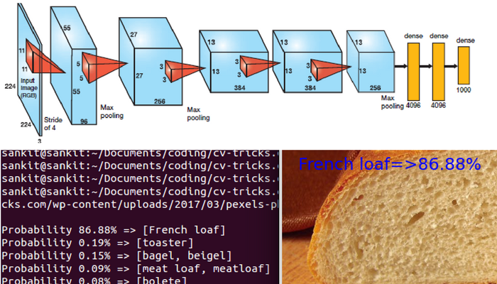
Alex Krizhevsky changed the world when he first won Imagenet challenged in 2012 using a convolutional neural network for image classification task. Alexnet achieved top-5 accuracy of 84.6% in the classification task while the team that stood second had top-5 accuracy of 73.8% which was a record breaking and unprecedented difference. Before this, CNNs (and the people who were working on it) were not so popular among computer vision community. However, the tables were turned after this. Soon, most of the computer vision researchers started working on CNN and the accuracy has improved significantly over last 4-5 years.
Alexnet has 5 convolutional layers which are followed by 3 fully connected layers. Alex trained it on 2 GPUs as computational capacity was quite limited back in 2012.

Architecture of Alexnet which won 2012 Imagenet challenge.
VGG was proposed by a reasearch group at Oxford in 2014. This network was once very popular due to its simplicity and some nice properties like it worked well on both image classification as well as detection tasks. However, If you are looking to build production systems in 2017 and someone suggests VGG, run. This is because the size of VGG network is too large(Imagenet pre-trained model is more than 500 MB) due to large fully connected layers. There are more accurate and less computationally efficient networks available.
VGG uses
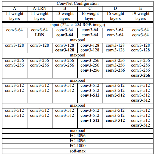
VGG and its variants: D and E were the most accurate and popular ones. They didn’t win Imagenet challenge in 2014 but were widely adopted due to simplicity
Alexnet was only 8 layers deep network, while VGG, ZFNet and other more accurate networks that followed had more layers. This proved that one needs to go deep to get higher accuracy, this is why this field got the name “Deep Learning”. However, proposed by a team at Google, Inception was the first architecture which improved results by design not by simply going deep.
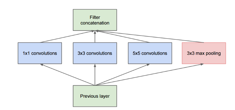
Naive inception module which was replaced by a sophisticated one later
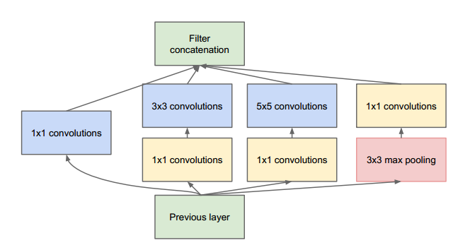
Refined Inception module
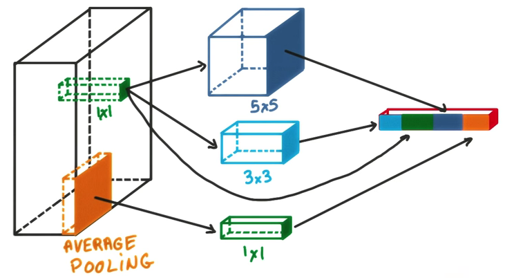
Inception module visualized: On the left is input which is “looked” in difference chunks and final output is a concatenation of all 3
iv) Resnet:
Microsoft won Imagenet challenge in 2015 by using 152 layer Resnet network which used a Resnet module:
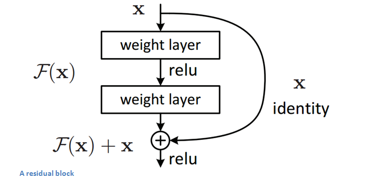
Resnet module proposed by Microsoft
They achieved 96.4% top-5 accuracy on Imagenet 2015. They also experimented with much deeper models like 1000 layer networks but accuracy droped with too deep models probably due to overfitting.
SqueezeNet is remarkable not for its accuracy but for how less computation does it need. Squeezenet has accuracy levels close to that of AlexNet however, the pre-trained model on Imagenet has a size of less than 5 MB which is great for using CNNs in a real world application. SqueezeNet introduced a Fire module which is made of alternate Squeeze and Expand modules.
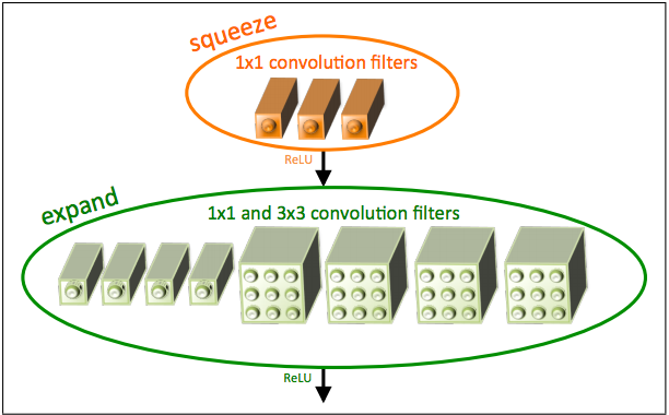
SqueezeNet fire module
With networks like SqueezeNet, it’s possible to reduce the amount of computation(hence, energy) required for similar kind of accuracy. “Given current power consumption by electronic computers, a computer with the storage and processing capability of the human mind would require in excess of 10 Terawatts of power, while human mind takes on 10 watts.” So, a lot of improvement is required in the efficiency of current neural networks and SqueezeNet is one step in that direction.
Great! you are now familiar with most of the popular and useful convolutional neural networks. In the next two sections, you shall run them on your own images.
a) From Tensorflow version 1.0 and above:
|
1 2 |
python -c "import tensorflow.contrib.slim as slim; eval = slim.evaluation.evaluate_once" |
b) For older versions:
If you happen to be running older version of Tensorflow and can’t upgrade for whatever reasons, install using following steps:
Go to the Jenkins page for Tensorflow project (where status of all the latest versions of Tensorflow are managed by Tensorflow team) and take the latest nightly(If you are not familiar with Jenkins, just google continuous integration).
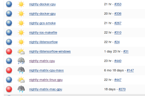
Jenkins for Tensorflow
Click on a relevant link, for example if you run ubuntu with gpu click on ‘nightly-matrix-linux-gpu’. On this page, you shall see a matrix for various python versions for PIP and NO_PIP versions. Choose NO_PIP with relevant python which will look like:
https://ci.tensorflow.org/view/All/job/nightly-matrix-linux-gpu/TF_BUILD_IS_OPT=OPT,TF_BUILD_IS_PIP=NO_PIP,TF_BUILD_PYTHON_VERSION=PYTHON2,label=gpu-linux/
Finally, append that with your relevant Tensorflow version .whl file. Now, install using:
|
1 2 3 4 |
export TF_BINARY_URL=https://ci.tensorflow.org/view/Nightly/job/nightly-matrix-linux-gpu/TF_BUILD_IS_OPT=OPT,TF_BUILD_IS_PIP=PIP,TF_BUILD_PYTHON_VERSION=PYTHON2,label=gpu-linux/lastSuccessfulBuild/artifact/pip_test/whl/tensorflow-0.11.0-cp27-none-linux_x86_64.whl sudo pip install --upgrade $TF_BINARY_URL |
Congratulations! This will install TF-Slim on your machine. To test your installation:
|
1 2 3 4 |
python >>import tensorflow as tf >>slim= tf.contrib.slim |
This should not throw any errors.
2.2) TensorFlow-Slim tutorial:
In order to import TF-Slim just do this:
|
1 2 |
slim = tf.contrib.slim |
2.2.1. Quick Slim variables
2.2.2. Higher level layers
2.2.3. Arg scope and using it
Let’s get started. Shall we?
|
1 2 3 4 5 6 |
weights = slim.variable('weights', shape=[10, 10, 3 , 3], initializer=tf.truncated_normal_initializer(stddev=0.1), regularizer=slim.l2_regularizer(0.05), device='/GPU:0') |
|
1 2 3 4 5 |
weights = slim.model_variable('weights', shape=[10, 10, 3 , 3], initializer=tf.truncated_normal_initializer(stddev=0.1, regularizer=slim.l2_regularizer(0.05), device='/CPU:0') |
regular_variables_and_model_variables = slim.get_variables()
|
1 2 3 |
input=... net = slim.conv2d(input, 128,[3, 3], scope='conv1_1') |
|
1 2 3 4 5 6 7 8 9 10 11 |
input = ... with tf.name_scope('conv1_1') as scope: kernel = tf.Variable(tf.truncated_normal([3, 3, 64,128], dtype=tf.float32, stddev=1e-1), name='weights') conv = tf.nn.conv2d(input, kernel,[1, 1, 1, 1], padding='SAME') biases = tf.Variable(tf.constant(0.0, shape=[128], dtype=tf.float32), trainable=True, name='biases') bias = tf.nn.bias_add(conv, biases) conv1 = tf.nn.relu(bias, name=scope) |
|
1 2 3 4 5 |
net = ... net = slim.conv2d(net, 256,[3, 3], scope='conv3_1') net = slim.conv2d(net, 256,[3, 3], scope='conv3_2') net = slim.conv2d(net, 256,[3, 3], scope='conv3_3') |
net = slim.repeat(net, 3, slim.conv2d, 256,[3, 3], scope='conv3')
|
1 2 3 4 |
x = slim.fully_connected(x, 32, scope='fc/fc_1') x = slim.fully_connected(x, 64, scope='fc/fc_2') x = slim.fully_connected(x, 128, scope='fc/fc_3') |
|
1 2 |
slim.stack(x, slim.fully_connected,[32, 64, 128], scope='fc') |
|
1 2 3 4 5 6 7 8 9 |
# Without stack: Verbose way: x = slim.conv2d(x, 32,[3, 3], scope='core/core_1') x = slim.conv2d(x, 32,[1, 1], scope='core/core_2') x = slim.conv2d(x, 64,[3, 3], scope='core/core_3') x = slim.conv2d(x, 64,[1, 1], scope='core/core_4') # Using stack: slim.stack(x, slim.conv2d,[(32,[3, 3]),(32,[1, 1]),(64,[3, 3]),(64,[1, 1])], scope='core') |
|
1 2 3 4 5 6 7 8 9 10 |
input = ... with tf.name_scope('conv1_1') as scope: kernel = tf.Variable(tf.truncated_normal([3, 3, 64, 128], dtype=tf.float32, stddev=1e-1), name='weights') conv = tf.nn.conv2d(input, kernel,[1, 1, 1, 1], padding='SAME') biases = tf.Variable(tf.constant(0.0, shape=[128], dtype=tf.float32), trainable=True, name='biases') bias = tf.nn.bias_add(conv, biases) conv1 = tf.nn.relu(bias, name=scope) |
|
1 2 3 4 5 6 7 8 9 10 |
net = slim.conv2d(inputs, 64,[11, 11], 4, padding='SAME', weights_initializer=tf.truncated_normal_initializer(stddev=0.01), weights_regularizer=slim.l2_regularizer(0.0005), scope='conv1') net = slim.conv2d(net, 128,[11, 11], padding='VALID', weights_initializer=tf.truncated_normal_initializer(stddev=0.01), weights_regularizer=slim.l2_regularizer(0.0005), scope='conv2') net = slim.conv2d(net, 256,[11, 11], padding='SAME', weights_initializer=tf.truncated_normal_initializer(stddev=0.01), weights_regularizer=slim.l2_regularizer(0.0005), scope='conv3') |
|
1 2 3 4 5 6 7 8 |
with slim.arg_scope([slim.conv2d], padding='SAME', weights_initializer=tf.truncated_normal_initializer(stddev=0.01) weights_regularizer=slim.l2_regularizer(0.0005)): net = slim.conv2d(inputs, 64,[11, 11], scope='conv1') net = slim.conv2d(net, 128,[11, 11], padding='VALID', scope='conv2') net = slim.conv2d(net, 256,[11, 11], scope='conv3') |
3.
|
1 2 3 |
inception_v1.ckpt 26 MB inception_v3.ckpt 104 MB |
The complete networks have been kept in nets folder. inception_v1.py and inception_v3.py are the files which define inception_v1 and inception_v3 networks respectively and we can build a network like this:
|
1 2 3 |
with slim.arg_scope(inception.inception_v1_arg_scope()): logits, _ = inception.inception_v1(processed_images, num_classes=1001, is_training=False) |
This will give the output of the last layer which can be converted to probabilities using softmax.
probabilities = tf.nn.softmax(logits)
Now, we have built our Tensorflow graph, the second step is to load the saved parameters in the network. For this, we shall use assign_from_checkpoint_fn function in which we shall specify the complete path of saved pre-trained model and all the variables we want to save. For inception_V1 network which has inceptionV1 as scope, we shall get all the model variables using slim.get_model_variables(‘InceptionV1’). Now we have created the graph and initialized the network parameters from the saved model, we can run the network inside a session:
|
1 2 3 4 |
with tf.Session() as sess: init_fn(sess) np_image, probabilities = sess.run([image, probabilities]) |
Finally, this will give out the index of labels, so we use imagenet.py inside dataset folder to get the mapping to print out the probabilities and show the results. Let’s Look at some of the results:
a). Inception_v1 result: Let’s run the prediction on this image of coffee:
|
1 2 |
python run_inference_on_v1.py https://cv-tricks.com/wp-content/uploads/2017/03/pexels-photo-362042.jpeg |
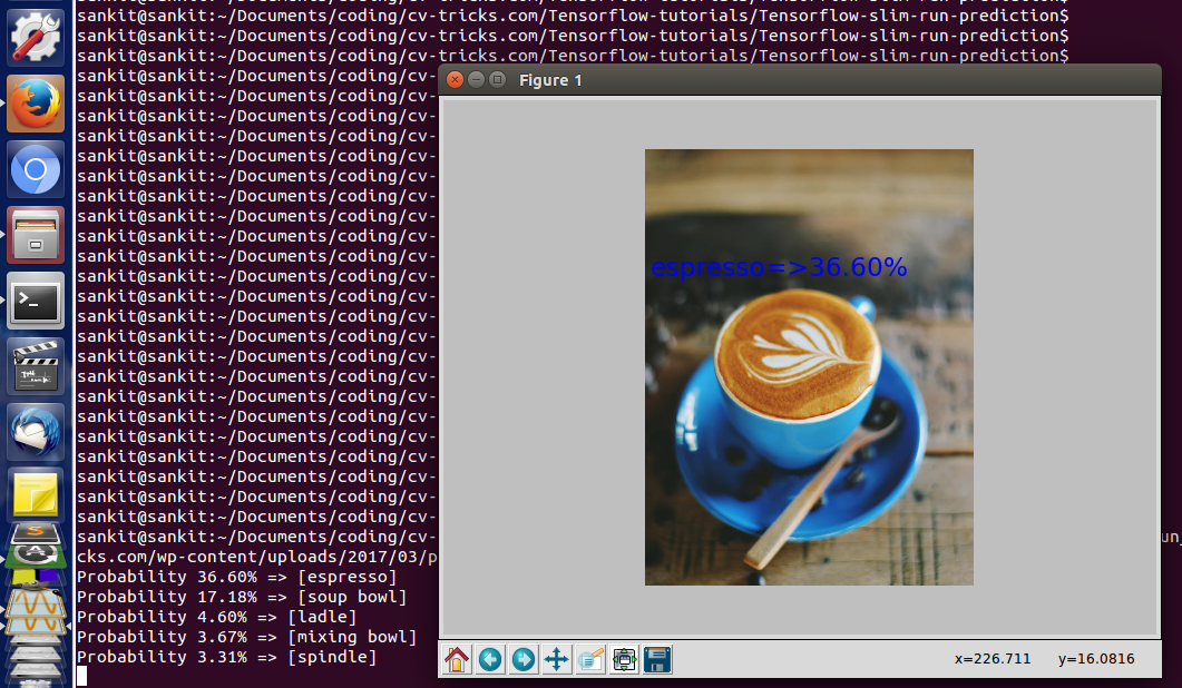
Inception_v1 identifies this image of expresso, however it is only 36% confident
Look at other results, some of them are are wrong but close like soup bowl.
b. Inception_v3 result: Let’s run inception_v3 which is much larger in size and more accurate.
|
1 2 |
python run_inference_on_v3.py https://cv-tricks.com/wp-content/uploads/2017/03/pexels-photo-280207.jpeg |

Prediction of inception_v3 on this image is spot-on and the model is very confident about it
This seems to be pretty good. Let’s run inception_v3 on the earlier image:
|
1 2 |
python run_inference_on_v3.py https://cv-tricks.com/wp-content/uploads/2017/03/pexels-photo-362042.jpeg |

