In a previous post, we covered various methods of object detection using deep learning. In this blog, I will cover Single Shot Multibox Detector in more details. SSD is one of the most popular object detection algorithms due to its ease of implementation and good accuracy vs computation required ratio.
Work proposed by Christian Szegedy is presented in a more comprehensible manner in the SSD paper https://arxiv.org/abs/1512.02325. This method, although being more intuitive than its counterparts like faster-rcnn, fast-rcnn(etc), is a very powerful algorithm. Being simple in design, its implementation is more direct from GPU and deep learning framework point of view and so it carries out heavy weight lifting of detection at lightning speed. Also, the key points of this algorithm can help in getting a better understanding of other state-of-the-art methods.
Here I have covered this algorithm in a stepwise manner which should help you grasp its overall working.
The breakdown of the post is as follows:
- General introduction to detection
- Sliding window detection
- Reducing redundant calculations of Sliding Window Method
- Training Methodology for modified network
- Dealing with Scale of the objects
1. Object detection and its relation to classification
Object detection is modeled as a classification problem. While classification is about predicting label of the object present in an image, detection goes further than that and finds locations of those objects too. In classification, it is assumed that object occupies a significant portion of the image like the object in figure 1.

figure 1

figure 2
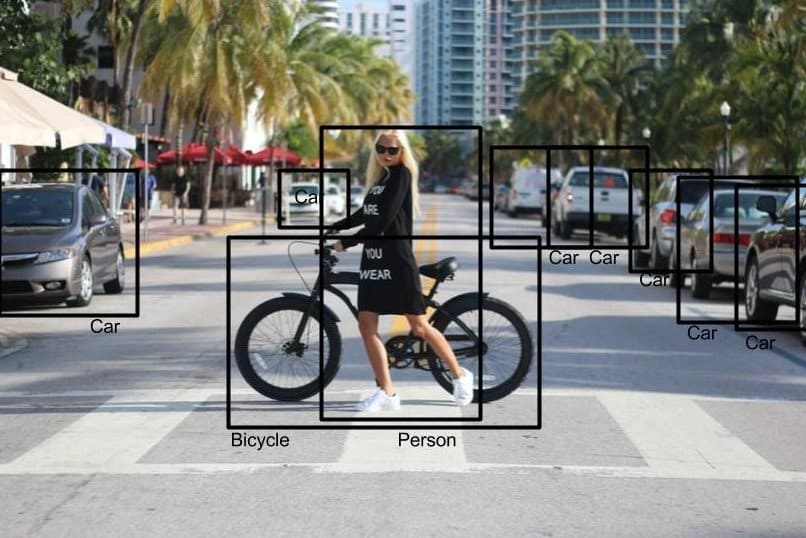
So the images(as shown in Figure 2), where multiple objects with different scales/sizes are present at different locations, detection becomes more relevant. So it is about finding all the objects present in an image, predicting their labels/classes and assigning a bounding box around those objects.
In image classification, we predict the probabilities of each class, while in object detection, we also predict a bounding box containing the object of that class. So, the output of the network should be:
- Class probabilities (like classification)
- Bounding box coordinates. We denote these by cx(x coordinate of center), cy(y coordinate of center), h(height of object), w(width of object)
Class probabilities should also include one additional label representing background because a lot of locations in the image do not correspond to any object.
For the sake of convenience, let’s assume we have a dataset containing cats and dogs. An image in the dataset can contain any number of cats and dogs. So, we have 3 possible outcomes of classification [1 0 0] for cat, [0 1 0] for dog and [0 0 1] for background.
Object Detection as Image Classification problem
A simple strategy to train a detection network is to train a classification network. This classification network will have three outputs each signifying probability for the classes cats, dogs, and background. For training classification, we need images with objects properly centered and their corresponding labels.
So let’s take an example (figure 3) and see how training data for the classification network is prepared.
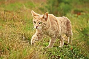
figure 3: Input image for object detection
In order to do that, we will first crop out multiple patches from the image. The following figure shows sample patches cropped from the image.
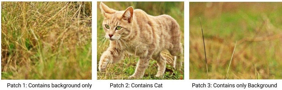
Various patches generated from input image above
The patch 2 which exactly contains an object is labeled with an object class. So we assign the class “cat” to patch 2 as its ground truth. If output probabilities are in the order cat, dog, and background, ground truth becomes [1 0 0]. Then for the patches(1 and 3) NOT containing any object, we assign the label “background”. Therefore ground truth for these patches is [0 0 1].
Now, this is how we need to label our dataset that can be used to train a convnet for classification.
2. Sliding Window Detector:
After the classification network is trained, it can then be used to carry out detection on a new image in a sliding window manner. First, we take a window of a certain size(blue box) and run it over the image(shown in Figure below) at various locations.
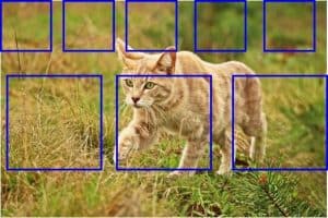
Then we crop the patches contained in the boxes and resize them to the input size of classification convnet. We then feed these patches into the network to obtain labels of the object. We repeat this process with smaller window size in order to be able to capture objects of smaller size. So the idea is that if there is an object present in an image, we would have a window that properly encompasses the object and produce label corresponding to that object. Here is a gif that shows the sliding window being run on an image:
But, how many patches should be cropped to cover all the objects? We will not only have to take patches at multiple locations but also at multiple scales because the object can be of any size. This will amount to thousands of patches and feeding each of them in a network will result in huge of amount of time required to make predictions on a single image.
So let’s look at the method to reduce this time.
3. Reducing redundant calculations to reduce time
Now let’s consider multiple crops shown in figure 5 by different colored boxes which are at nearby locations.
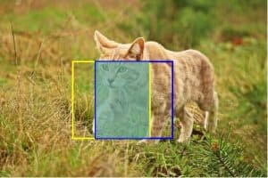
figure 5
We can see there is a lot of overlap between these two patches(depicted by shaded region). This means that when they are fed separately(cropped and resized) into the network, the same set of calculations for the overlapped part is repeated. This can easily be avoided using a technique which was introduced in SPP-Net and made popular by Fast R-CNN. Let’s take an example network to understand this in details.
The following figure-6 shows an image of size 12X12 which is initially passed through 3 convolutional layers, each with filter size 3×3(with varying stride and max-pooling). Notice that, after passing through 3 convolutional layers, we are left with a feature map of size 3x3x64 which has been termed penultimate feature map i.e. feature map just before applying classification layer. We name this because we are going to be referring it repeatedly from here on. On top of this 3X3 map, we have applied a convolutional layer with a kernel of size 3X3. Three sets of this 3X3 filters are used here to obtain 3 class probabilities(for three classes) arranged in 1X1 feature map at the end of the network.
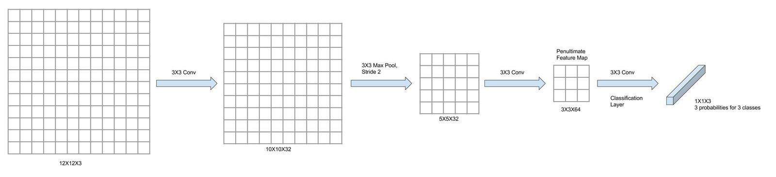
Figure-6
Now, we shall take a slightly bigger image to show a direct mapping between the input image and feature map. Let’s increase the image to 14X14(figure 7). We can see that 12X12 patch in the top left quadrant(center at 6,6) is producing the 3×3 patch in penultimate layer colored in blue and finally giving 1×1 score in final feature map(colored in blue). The second patch of 12X12 size from the image located in top right quadrant(shown in red, center at 8,6) will correspondingly produce 1X1 score in final layer(marked in red).
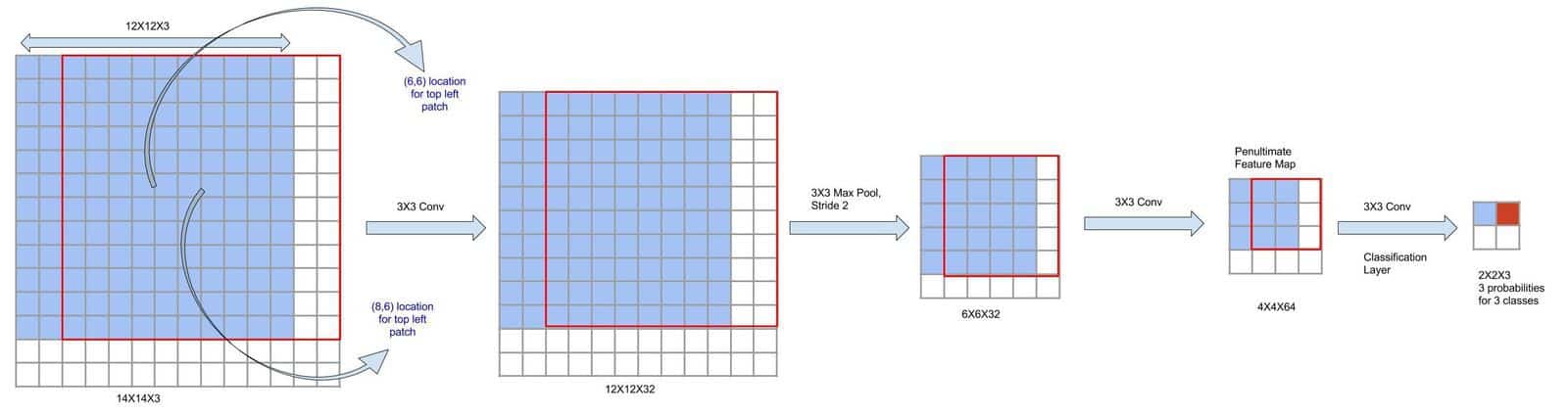
Figure 7: Depicting overlap in feature maps for overlapping image regions
As you can see, different 12X12 patches will have their different 3X3 representations in the penultimate map and finally, they produce their corresponding class scores at the output layer.
Calculating convolutional feature map is computationally very expensive and calculating it for each patch will take very long time. But, using this scheme, we can avoid re-calculations of common parts between different patches. Here we are calculating the feature map only once for the entire image. And then since we know the parts on penultimate feature map which are mapped to different paches of image, we direcltly apply prediction weights(classification layer) on top of it. It is like performing sliding window on convolutional feature map instead of performing it on the input image. So this saves a lot of computation.
To summarize we feed the whole image into the network at one go and obtain feature at the penultimate map. And then we run a sliding window detection with a 3X3 kernel convolution on top of this map to obtain class scores for different patches.
There is a minor problem though. Not all patches from the image are represented in the output. In our example, 12X12 patches are centered at (6,6), (8,6) etc(Marked in the figure). Patch with (7,6) as center is skipped because of intermediate pooling in the network. In a moment, we will look at how to handle these type of objects/patches.
Default Boxes/Anchor Boxes
So the boxes which are directly represented at the classification outputs are called default boxes or anchor boxes. In the above example, boxes at center (6,6) and (8,6) are default boxes and their default size is 12X12. Note that the position and size of default boxes depend upon the network construction.
4. Training Methodology for modified network
Let’s see how we can train this network by taking another example. Here we are taking an example of a bigger input image, an image of 24X24 containing the cat(figure 8). It is first passed through the convolutional layers similar to above example and produces an output feature map of size 6×6.

Figure 8
For preparing training set, first of all, we need to assign the ground truth for all the predictions in classification output. Let us index the location at output map of 7,7 grid by (i,j). We already know the default boxes corresponding to each of these outputs. For reference, output and its corresponding patch are color marked in the figure for the top left and bottom right patch. Now since patch corresponding to output (6,6) has a cat in it, so ground truth becomes [1 0 0]. Since the patches at locations (0,0), (0,1), (1,0) etc do not have any object in it, their ground truth assignment is [0 0 1].
The patches for other outputs only partially contains the cat. Let us see how their assignment is done.
Ground truth Assignment for partially covered patches
To understand this, let’s take a patch for the output at (5,5). The extent of that patch is shown in the figure along with the cat(magenta). We can see that the object is slightly shifted from the box. The box does not exactly encompass the cat, but there is a decent amount of overlap.
So for its assignment, we have two options: Either tag this patch as one belonging to the background or tag this as a cat. Tagging this as background(bg) will necessarily mean only one box which exactly encompasses the object will be tagged as an object. And all the other boxes will be tagged bg. This has two problems. Firstly the training will be highly skewed(large imbalance between object and bg classes). Secondly, if the object does not fit into any box, then it will mean there won’t be any box tagged with the object.
So we resort to the second solution of tagging this patch as a cat. But in this solution, we need to take care of the offset in center of this box from the object center. Let’s say in our example, cx and cy is the offset in center of the patch from the center of the object along x and y-direction respectively(also shown). We need to devise a way such that for this patch, the network can also predict these offsets which can thus be used to find true coordinates of an object.
So for every location, we add two more outputs to the network(apart from class probabilities) that stands for the offsets in the center. Let’s call the predictions made by the network as ox and oy. And in order to make these outputs predict cx and cy, we can use a regression loss. Vanilla squared error loss can be used for this type of regression. The papers on detection normally use smooth form of L1 loss. We will skip this minor detail for this discussion.
5. Dealing with Scale changes
Now that we have taken care of objects at different locations, let’s see how the changes in the scale of an object can be tackled.
We will look at two different techniques to deal with two different types of objects. One type refers to the object whose size is somewhere near to 12X12 pixels(default size of the boxes). The other type refers to the objects whose size is significantly different from 12X12.
Objects with size close to 12X12
For the objects similar in size to 12X12, we can deal them in a manner similar to the offset predictions. Let us assume that true height and width of the object is h and w respectively. So we add two more dimensions to the output signifying height and width(oh, ow). Then we again use regression to make these outputs predict the true height and width.
Objects far smaller than 12X12
Dealing with objects very different from 12X12 size is a little trickier. For the sake of argument, let us assume that we only want to deal with objects which are far smaller than the default size.
The one line solution to this is to make predictions on top of every feature map(output after each convolutional layer) of the network as shown in figure 9. The prediction layers have been shown as branches from the base network in figure. This is the key idea introduced in Single Shot Multibox Detector. Let us understand this in detail.
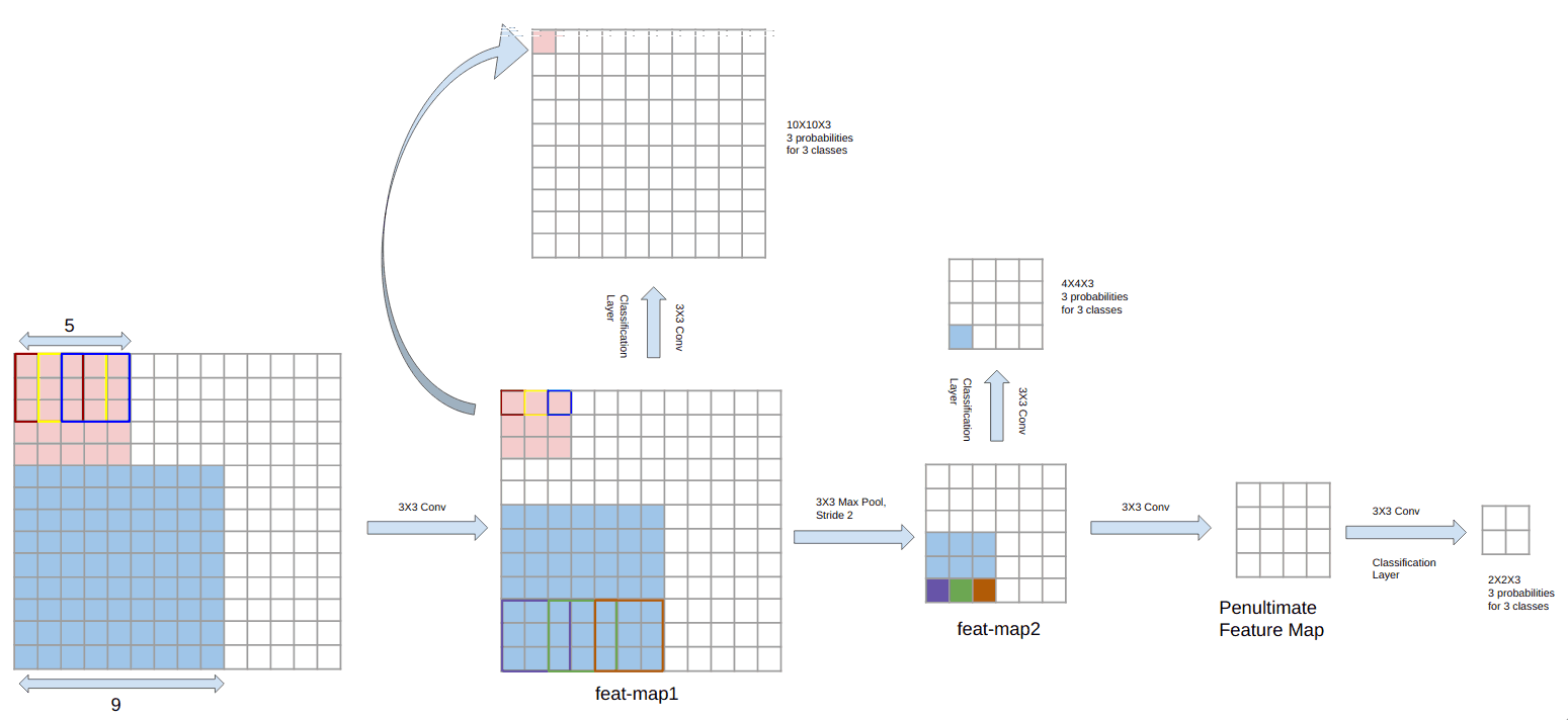
figure 9
Using all feature maps for predictions
Earlier we used only the penultimate feature map and applied a 3X3 kernel convolution to get the outputs(probabilities, center, height, and width of boxes). Here we are applying 3X3 convolution on all the feature maps of the network to get predictions on all of them. Predictions from lower layers help in dealing with smaller sized objects. How is it so?
Remember, conv feature map at one location represents only a section/patch of an image. That is called its receptive field size. We have seen this in our example network where predictions on top of penultimate map were being influenced by 12X12 patches.
Convolutional networks are hierarchical in nature. And each successive layer represents an entity of increasing complexity and in doing so, their receptive field on input image increases as we go deeper. So predictions on top of penultimate layer in our network have maximum receptive field size(12X12) and therefore it can take care of larger sized objects. And shallower layers bearing smaller receptive field can represent smaller sized objects.
In our sample network, predictions on top of first feature map have a receptive size of 5X5 (tagged feat-map1 in figure 9). It can easily be calculated using simple calculations. It has been explained graphically in the figure. Similarly, predictions on top of feature map feat-map2 take a patch of 9X9 into account. So we can see that with increasing depth, the receptive field also increases.
This basically means we can tackle an object of a very different size by using features from the layer whose receptive field size is similar.
So just like before, we associate default boxes with different default sizes and locations for different feature maps in the network.
Now during the training phase, we associate an object to the feature map which has the default size closest to the object’s size. So for example, if the object is of size 6X6 pixels, we dedicate feat-map2 to make the predictions for such an object. Therefore we first find the relevant default box in the output of feat-map2 according to the location of the object. And then we assign its ground truth target with the class of object. This technique ensures that any feature map do not have to deal with objects whose size is significantly different than what it can handle. And thus it gives more discriminating capability to the network.
This way we can now tackle objects of sizes which are significantly different than 12X12 size.
Conclusion
This concludes an overview of SSD from a theoretical standpoint. There are few more details like adding more outputs for each classification layer in order to deal with objects not square in shape(skewed aspect ratio). Also, SSD paper carves out a network from VGG network and make changes to reduce receptive sizes of layer(atrous algorithm). I hope all these details can now easily be understood from referring the paper.