GhostNetV2 is a recent SOTA architecture that allows an implementation of Long-Range attention in the deep CNN frameworks used in various ML tasks such as image classification, object detection, and video analysis. GhostNetV2 proposes a new attention mechanism called DFC attention to capture long range spatial information. And it does so while keeping the implementation efficiency of light-weight convolutional neural networks suitable for deployment on edge devices like smartphone and wearables.
The main component of GhostNetV2 is the GhostV2 module. The main building component of which are the Ghost module and DFC attention. Below, we look at these components to understand the architecture of GhostNetV2.
Ghost Module
Abundant and even redundant information in the feature maps of well-trained deep neural networks often guarantees a comprehensive understanding of the input data. For example, the figure below presents some feature maps of an input image generated by ResNet-50. From the figure, we can see that there exists many similar pairs of feature maps, like a ghost of another. Thus, redundancy in feature maps could be an important characteristic for a successful deep neural network. The Ghost module exploits this redundancy to do convolution in Neural Networks in a cost efficient way by reducing the number of convolution filters required to generate them.

Visualization of some feature maps generated by the first
residual group in ResNet-50. Similar feature map pair
examples are annotated with boxes of the same color. One feature
map in the pair can be approximately obtained by transforming the
other one through cheap operations (denoted by spanners)
An arbitrary convolution operation can be represented as follows:
\( Y = X * f + b \)
where \( X \in \mathbb{R}^{c \times h \times w} \) is the input features with height h, width w and #channels c; \( Y \in \mathbb{R}^{h’ \times w’ \times n} \) is the output with n features; \( b \) denotes the bias term; and \( f \in \mathbb{R}^{c \times k \times k \times n} \) denotes the convolution filters with kernel size \( k \times k \). The Ghost module replaces this operation with two sequential operations : a primary convolution and a secondary step.
Exploiting the aforementioned redundancy, the primary convolution generates a small set of intrinsic features which are then used by the secondary step to generate the feature maps similar to the original convolution. For input \( X \), the small set of intrinsic feature maps, \( Y’ \), is generated as:
\( Y’ = X * f’ + b’ \)where \( Y’ \in \mathbb{R}^{h’ \times w’ \times m} \) ( \( m \leq n\) ), and \( f’ \in \mathbb{R}^{c \times k \times k \times m} \). The hyperparameters such as filter size, stride and padding are kept the same as those in the ordinary convolution. Now to further obtain the desired n feature maps the paper applies a series of cheap linear operations on each intrinsic feature in \(Y’\),
![]()
where \( \Phi_{i,j} \) is a cheap linear operation for generating the \( j^{th} \) ghost feature map from the \( i^{th} \) intrinsic feature \( y_i^\prime \). Here the last \( \Phi_{i,s} \) is taken to be an identity map.
Taking \( n=m \cdot s\), the number of output features for the Ghost module can be kept the same as the original number of features. In practice the linear operation \( \Phi_{i,j} \) could contain several different linear operations e.g. 3×3 and 5×5 linear kernels.
The number of FLOPs required for the original convolution operation is \( n \cdot h^\prime \cdot w^\prime \cdot c \cdot k \cdot k \). Thus, the theoretical speed-up ratio of upgrading ordinary convolution with the Ghost module is,

where d × d has the similar magnitude as that of k × k, and \( s\ll c\).
The second main component of the Ghost Module is the attention mechanism added to the Ghost module. Let us now look at the new attention mechanism dubbed Decoupled Fully Connected (DFC) attention.
DFC Attention
In GhostNetv2, the authors upgrade the Ghost module with an attention mechanism, called DFC attention, to make the GhostV2 module. The attention map for the new attention mechanism is generated in a novel manner to keep the module computationally efficient. Let us now describe the generation of this attention map (figure below).

Module for generating the attention map for Decoupled Fully Connected (DFC) attention mechanism
Given an input feature \( Z \in \mathbb{R}^{C \times H \times W} \), it can be written as \( H \cdot W \) tokens \( \mathbf{z}_{h w} \in \mathbb{R}^C \). Now, a direct implementation of a fully connected layer to generate the attention map can be written as:

where F denotes the learnable weights, \( \mathbf{a}_{hw} \) denotes the attention maps, and \( \odot \) denotes element-wise multiplication. This is a much simpler implementation of attention, but the computational complexity of this computation is quadratic i.e. \( \mathcal{O}(H^2W^2) \). That makes this attention mechanism impractical especially for high resolution images. So, the paper decomposes the fully connected attention above into two fully connected layers, as follows:

where \( F^H \) and \( F^W \) are learnable transformation weights. Note that in this decomposition, a patch is directly aggregated by patches in its vertical/horizontal lines, while other patches participate in the generation of those patches in the vertical/horizontal lines, having an indirect relationship with the focused token. Thus the calculation of a patch involves all the patches in the square region.
The decomposition above can be conveniently, implemented using convolution operations leaving out the time-consuming tensor reshaping and transposing operations. And instead of filters of image sizes we can use fixed length (\( 1\times K_H \) & \( K_W\times1 \)) filters to allow processing of input images with varying resolutions. Thus, the theoretical complexity of DFC attention becomes \( \mathcal{O}(K_H HW + K_W HW) \), as compared to the quadratic complexity of self-attention, \( \mathcal{O}(H^2W^2) \).
Ghostv2 Module
The GhostV2 module enhances Ghost module’s output to capture long-range dependence among different spatial pixels using DFC attention. For an input feature \( X \in \mathbb{R}^{H\times W\times C} \), let us denote the output of the Ghost module with \( Y \). A \( 1 \times 1\) convolution is used to convert the input \(X\) to the input to DFC attention module, \( Z \), similar to the linear layer for generating the Query and Keys in regular self attention. The attention map output from the DFC module is denoted by \(A\). Then, the Output \( O \) of the module is the element-wise product of the two outputs ie
\( O = Sigmoid(A) \odot Y \)where Sigmoid is used to normalize the attention map A into range (0,1).

GhostV2 Module
Note that in practice the DFC attention is computed on down-sampled version of input features \( X \), to save on computational resources. An upsampled ouput –using bilinear interpolation– \( Sigmoid(A) \) is then fed to the element-wise multiplication operation above.
GhostNetV2 (and GhostNetV1)
The version 1 of GhostNet creates a Ghost bottleneck module (figure below) using the Ghost module. GhostNet basically follow the architecture of MobileNetV3 and replaces the bottleneck block in MobileNetV3 with the Ghost bottleneck.

GhostV1 bottleneck
The Ghost bottleneck appears to be similar to the basic residual block in ResNet. It mainly consists of two stacked Ghost modules. The first Ghost module acts as an expansion layer increasing the number of channels while the second Ghost module reduces the number of channels to match the shortcut path. In the ghost bottleneck for stride 2, the shortcut path is implemented by a downsampling layer and a depthwise convolution with stride=2 is inserted between the two Ghost modules.
GhostNetV2 also follows the MobileNetV3 architecture. It uses the GhostV2 bottleneck (figure below) to replace the bottleneck block in MobileNetv3. We can see that the GhostV2 bottleneck replaces only the first Ghost module with the GhostV2 module. The authors justify this with empirical results which show that replacing the second ghost module does not provide as much improvement in the performance in exchange for the increased number of FLOPs.

GhostV2 bottleneck
Here is the performance of GhostNetv2 compared to other lightweight architectures, on the Imagenet dataset

Top-1 accuracy vs FLOPs and Latency on the Imagenet dataset