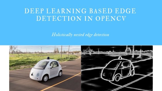
In this post, we will learn how to use deep learning based edge detection in OpenCV which is more accurate than the widely popular canny edge detector. Edge detection is useful in many use-cases such as visual saliency detection, object detection, tracking and motion analysis, structure from motion, 3D reconstruction, autonomous driving, image to text analysis and many more.
What is Edge Detection?
Edge detection is a very old problem in computer vision which involves detecting the edges in an image to determine object boundary and thus separate the object of interest. One of the most popular technique for edge detection has been Canny Edge detection which has been the go-to method for most of the computer vision researchers and practitioners. Let’s have a quick look at Canny Edge Detection.
Canny Edge Detection Algorithm:
Canny Edge detection was invented by John Canny in 1983 at MIT. It treats edge detection as a signal processing problem. The key idea is that if you observe the change in intensity on each pixel in an image, it’s very high on the edges.
In this simple image below, the intensity change only happens on the boundaries. So, you can very easily identify edges just by observing the change in intensity.
![]()
Now, look at this image. The intensity is not constant but the rate of change in intensity is highest at the edges. (Calculus refresher: The rate of change can be calculated using the first derivative(gradient).)

The Canny Edge Detector identifies edges in 4 steps:
- Noise removal: Since this method depends on sudden changes in intensity and if the image has a lot of random noise, then it would detect that as an edge. So, it’s a very good idea to smoothen your image using a Gaussian filter of 5×5.
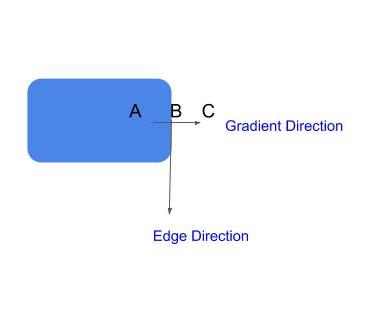
- Gradient Calculation: In the next step, we calculate the gradient of intensity(rate of change in intensity) on each pixel in the image. We also calculate the direction of the gradient.

Gradient direction is perpendicular to the edges. It’s mapped to one of the four directions(horizontal, vertical, and two diagonal directions).
3. Non-Maximal Suppression:
Now, we want to remove the pixels(set their values to 0) which are not edges. You would say that we can simply pick the pixels with the highest gradient values and those are our edges. However, in real-world images, gradient doesn’t simply peak at one pixel, rather it’s very high on the pixels near the edge as well. So, we pick the local maxima in a neighborhood of 3×3 in the direction of gradients.
4. Hysteresis Thresholding:
In the next step, we need to decide on a threshold value of the gradient below which all the pixels would be suppressed(set to zero). However, Canny edge detector using Hysteresis thresholding. Hysteresis thresholding is one of the very simple yet powerful ideas. It says that in place of using just one threshold we would use two thresholds:
High threshold= A very high value is chosen in such a way that any pixel having gradient value higher than this value is definitely an edge.
Low threshold= A low value is chosen in such a way that any pixel having gradient value below this value is definitely not an edge.
Pixels having gradients between these two thresholds are checked if they are connected to an edge, if yes, then they are kept else suppressed.
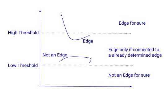
Hysteresis thresholding
Problem with Canny Edge detector:
Since the Canny edge detector only focuses on local changes and it has no semantic(understanding the content of the image) understanding, it has limited accuracy(which is great a lot of times).
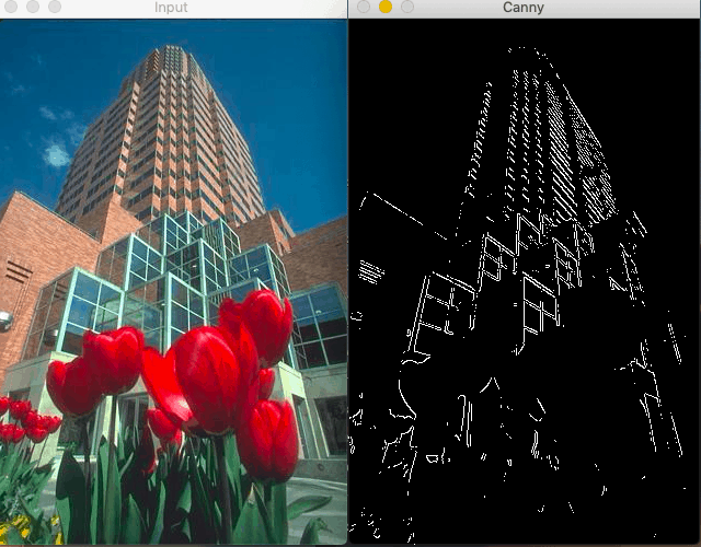
Canny Edge detector fails in this case as it has no understanding of the content of the image.
Semantic understanding is crucial for edges detection that is why learning based detectors which use machine learning or deep learning generate better results than canny edge detector.
Deep Learning based Edge Detection in OpenCV:
OpenCV has integrated a deep learning based edge detection technique in its new fancy DNN module. You would need version OpenCV version 3.4.3 or higher. This technique called holistically nested edge detection or HED is a learning-based end-to-end edge detection system that uses a trimmed VGG-like convolutional neural network for an image to image prediction task.
HED makes use of the side outputs of intermediate layers. The output of earlier layers is called side output and the output of all 5 convolutional layers is fused to generate the final predictions. Since the feature maps generated at each layer is of different size, it’s effectively looking at the image at different scales.
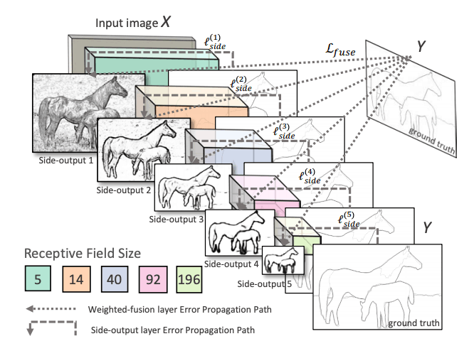
Network Architecture: Holistically nested Edge detection: Figure from the paper
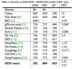
HED method is not only more accurate than other deep learning based methods but also much faster than them too. That’s why OpenCV has decided to integrate this into the new DNN module. Here are the results from the paper:
Code for running DL Edge Detection in OpenCV:
The pre-trained model that OpenCV uses has been trained in Caffe framework which can be downloaded by running:
|
1 2 |
sh download_pretrained.sh |
There is a Crop layer that this network uses which is not implemented by default so we need to provide our own implementation of this layer.
|
1 2 3 4 5 6 7 8 9 10 11 12 13 14 15 16 17 18 19 20 21 22 23 24 |
class CropLayer(object): def __init__(self, params, blobs): self.xstart = 0 self.xend = 0 self.ystart = 0 self.yend = 0 # Our layer receives two inputs. We need to crop the first input blob # to match a shape of the second one (keeping batch size and number of channels) def getMemoryShapes(self, inputs): inputShape, targetShape = inputs[0], inputs[1] batchSize, numChannels = inputShape[0], inputShape[1] height, width = targetShape[2], targetShape[3] self.ystart = (inputShape[2] - targetShape[2]) // 2 self.xstart = (inputShape[3] - targetShape[3]) // 2 self.yend = self.ystart + height self.xend = self.xstart + width return [[batchSize, numChannels, height, width]] def forward(self, inputs): return [inputs[0][:,:,self.ystart:self.yend,self.xstart:self.xend]] |
Now, we can simply register this layer with a single line of code by passing it the over-ridding class.
cv.dnn_registerLayer('Crop', CropLayer)
Now, we are ready to build the network graph and load the weights which can be done via OpenCV’s dnn.readNet function.
net = cv.dnn.readNet(args.prototxt, args.caffemodel)
Now the next step is to load images in a batch and run them through the network. For this, we use the cv2.dnn.blobFromImage method. This method creates 4-dimensional blob from input images. Let’s look at the signature of this method:
blob = cv.dnn.blobFromImage(image, scalefactor, size, mean, swapRB, crop)
Where:
image: is the input image that we want to send to the neural network for inference.
scalefactor: If we want to scale our images by multiplying them by a constant number. A lot of times we divide all of our uint8 images by 255, this way all the pixels are between 0 and 1(0/255-255/255). The default value is 1.0 which is no scaling.
size: The spatial size of the output image. It will be equal to the input size required for the follow-on neural networks as the output of blobFromImage.
swapRB: Boolean to indicate if we want to swap the first and last channel in 3 channel image. OpenCV assumes that images are in BGR format by default but if we want to swap this order to RGB, we can set this flag to True which is also the default.
mean: In order to handle intensity variations and normalization, sometimes we calculate the average pixel value on the training dataset and subtract it from each image during training. If we are doing mean subtraction during training, then we must apply it during inference. This mean will be a tuple corresponding to R, G, B channels. For example mean values on the Imagenet dataset is R=103.93, G=116.77, and B=123.68. If we use swapRB=False, then this order will be (B, G, R).
crop: Boolean flag to indicate if we want to center crop our images. If it’s set to True, the input image is cropped from the center in such a way that smaller dimension is equal to the corresponding dimension in size and other dimension is equal or larger. However, if we set it to False, it would preserve the aspect ratio and just resize to dimensions in size.
In our case:
|
1 2 3 4 |
inp = cv.dnn.blobFromImage(frame, scalefactor=1.0, size=(args.width, args.height), mean=(104.00698793, 116.66876762, 122.67891434), swapRB=False, crop=False) |
Now, we just need to call the forward method.
|
1 2 3 4 5 6 7 8 9 10 |
net.setInput(inp) out = net.forward() out = out[0, 0] out = cv.resize(out, (frame.shape[1], frame.shape[0])) out = 255 * out out = out.astype(np.uint8) out=cv.cvtColor(out,cv.COLOR_GRAY2BGR) con=np.concatenate((frame,out),axis=1) cv.imshow(kWinName,con) |
And Here are a few results:
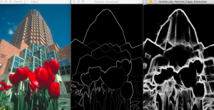
Results: Middle image is the human annotated image, the right one is the result of HED

Results: Middle image is the human annotated image, the right one is the result of HED
The code for this blog post can be downloaded from our GitHub repository here.
