4.1) Solve a linear regression problem with example
1. Why Keras?
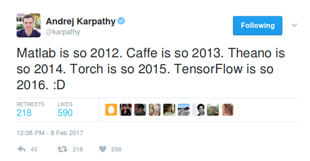
Currently, Keras is one of the fastest growing libraries for deep learning.
Install h5py for saving and restoring models:
|
1 2 |
pip install h5py |
Other python dependencies need to be installed.
|
1 2 3 |
pip install numpy scipy pip install pillow |
|
1 2 |
sudo pip install keras |
Checking the Keras version.
|
1 2 3 4 |
>>python -c "import keras; print(keras.__version__)" Using TensorFlow backend. 2.0.1 |
|
1 2 3 4 5 6 7 |
{ "epsilon": 1e-07, "floatx": "float32", "image_data_format": "channels_last", "backend": "tensorflow" } |
|
1 2 |
import keras |
Keras has two distinct ways of building models:
- In the next sections of this blog, you would understand the theory and examples of Keras Sequential Model and functional API.
This is how we start by importing and building a Sequential model.
|
1 2 3 |
from keras.models import Sequential model = Sequential() |
We can add layers like Dense(fully connected layer), Activation, Conv2D, MaxPooling2D etc by calling add function.
|
1 2 3 4 |
from keras.layers import Dense, Activation,Conv2D,MaxPooling2D,Flatten,Dropout model.add(Conv2D(64, (3, 3), activation='relu')) // This adds a Convolutional layer with 64 filters of size 3 * 3 to the graph |
1. Convolutional layer: Here, we shall add a layer with 64 filters of size 3*3 and use relu activations after that.
|
1 2 |
model.add(Conv2D(64, (3, 3), activation='relu')) |
2. MaxPooling layer: Specify the type of layer and specify the pool size and you are done. How cool is that!
|
1 2 |
model.add(MaxPooling2D(pool_size=(2, 2))) |
|
1 2 |
model.add(Dense(256, activation='relu')) |
|
1 2 |
model.add(Dropout(0.5)) |
|
1 2 |
model.add(Flatten()) |
|
1 2 |
model.add(Conv2D(32, (3, 3), activation='relu', input_shape=(224, 224, 3))) |
the
|
1 2 3 |
model.compile(loss='binary_crossentropy', optimizer='rmsprop') |
If you want to specify stochastic gradient descent and you want to choose proper initialization and other hyperparameters:
|
1 2 3 4 5 6 |
from keras.optimizers import SGD ....... ...... sgd = SGD(lr=0.01, decay=1e-6, momentum=0.9, nesterov=True) model.compile(loss='categorical_crossentropy', optimizer=sgd) |
|
1 2 |
model.fit(x_train, y_train, batch_size=32, epochs=10,validation_data=(x_val, y_val)) |
|
1 2 |
score = model.evaluate(x_test, y_test, batch_size=32) |
These are the basic building blocks to use the Sequential model in Keras. Now, let’s build a simple example to implement linear regression using Keras Sequential model.
|
1 2 3 4 5 6 7 8 |
import keras from keras.models import Sequential from keras.layers import Dense import numpy as np trX = np.linspace(-1, 1, 101) trY = 3 * trX + np.random.randn(*trX.shape) * 0.33 |
b) Create model:
|
1 2 3 |
model = Sequential() model.add(Dense(input_dim=1, output_dim=1, init='uniform', activation='linear')) |
This will take input x and apply weight, w, and bias, b followed by a linear activation to produce output.
|
1 2 3 4 5 6 |
weights = model.layers[0].get_weights() w_init = weights[0][0][0] b_init = weights[1][0] print('Linear regression model is initialized with weights w: %.2f, b: %.2f' % (w_init, b_init)) ## Linear regression model is initialized with weight w: -0.03, b: 0.00 |
Now, we shall train this linear model with our training data of trX and trY, where trY is 3 times of trX, so this value of weights should become 3.
|
1 2 |
model.compile(optimizer='sgd', loss='mse') |
Finally, we feed the data using fit function
|
1 2 |
model.fit(trX, trY, nb_epoch=200, verbose=1) |
Now, we print the weight after training:
|
1 2 3 4 5 6 7 |
weights = model.layers[0].get_weights() w_final = weights[0][0][0] b_final = weights[1][0] print('Linear regression model is trained to have weight w: %.2f, b: %.2f' % (w_final, b_final)) ##Linear regression model is trained to have weight w: 2.94, b: 0.08 |
HDF5 Binary format:
|
1 2 |
model.save_weights("my_model.h5") |
Restoring pre-trained weights:
|
1 2 |
model.load_weights('my_model_weights.h5') |
6. Functional API:
|
1 2 |
from keras.models import Model |
|
1 2 |
from keras.layers import Input |
|
1 2 |
digit_input = Input(shape=(28, 28,1)) |
|
1 2 3 4 5 |
x = Conv2D(64, (3, 3))(digit_input) x = Conv2D(64, (3, 3))(x) x = MaxPooling2D((2, 2))(x) out = Flatten()(x) |
Finally, we create a model by specifying the input and output.
|
1 2 |
vision_model = Model(digit_input, out) |
Of course, one will also need to specify the loss, optimizer etc. using fit and compile methods, same as we did for the Sequential models.
Let’s just use what we have just learned and build a vgg-16 neural network. It’s a rather old and large network but is great for learning things due to its simplicity.
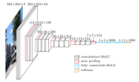
Vgg 16 architecture
|
1 2 3 4 5 6 7 8 9 10 11 12 13 14 15 16 17 18 19 20 21 22 23 24 25 26 27 28 29 30 31 32 33 34 |
img_input = Input(shape=input_shape) # Block 1 x = Conv2D(64, (3, 3), activation='relu', padding='same', name='block1_conv1')(img_input) x = Conv2D(64, (3, 3), activation='relu', padding='same', name='block1_conv2')(x) x = MaxPooling2D((2, 2), strides=(2, 2), name='block1_pool')(x) # Block 2 x = Conv2D(128, (3, 3), activation='relu', padding='same', name='block2_conv1')(x) x = Conv2D(128, (3, 3), activation='relu', padding='same', name='block2_conv2')(x) x = MaxPooling2D((2, 2), strides=(2, 2), name='block2_pool')(x) # Block 3 x = Conv2D(256, (3, 3), activation='relu', padding='same', name='block3_conv1')(x) x = Conv2D(256, (3, 3), activation='relu', padding='same', name='block3_conv2')(x) x = Conv2D(256, (3, 3), activation='relu', padding='same', name='block3_conv3')(x) x = MaxPooling2D((2, 2), strides=(2, 2), name='block3_pool')(x) # Block 4 x = Conv2D(512, (3, 3), activation='relu', padding='same', name='block4_conv1')(x) x = Conv2D(512, (3, 3), activation='relu', padding='same', name='block4_conv2')(x) x = Conv2D(512, (3, 3), activation='relu', padding='same', name='block4_conv3')(x) x = MaxPooling2D((2, 2), strides=(2, 2), name='block4_pool')(x) # Block 5 x = Conv2D(512, (3, 3), activation='relu', padding='same', name='block5_conv1')(x) x = Conv2D(512, (3, 3), activation='relu', padding='same', name='block5_conv2')(x) x = Conv2D(512, (3, 3), activation='relu', padding='same', name='block5_conv3')(x) x = MaxPooling2D((2, 2), strides=(2, 2), name='block5_pool')(x) x = Flatten(name='flatten')(x) x = Dense(4096, activation='relu', name='fc1')(x) x = Dense(4096, activation='relu', name='fc2')(x) x = Dense(classes, activation='softmax', name='predictions')(x) |
The complete code is provided in vgg16.py.
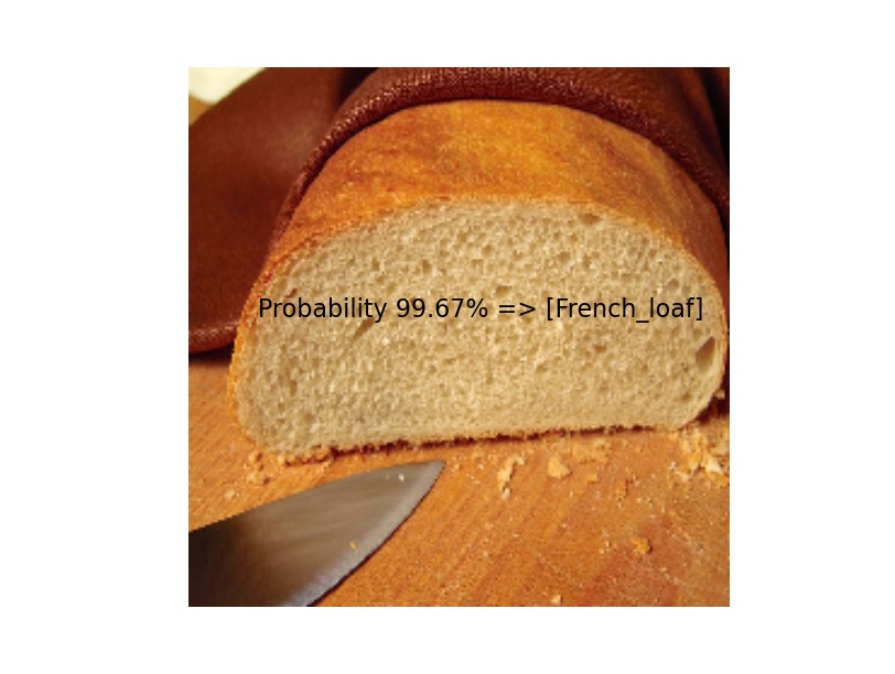
In this example, let’s run imageNet predictions on some images. Let’s write the code for the same:
|
1 2 3 4 5 6 7 8 9 10 |
model = applications.VGG16(weights='imagenet') img = image.load_img('cat.jpeg', target_size=(224, 224)) x = image.img_to_array(img) x = np.expand_dims(x, axis=0) x = preprocess_input(x) preds = model.predict(x) for results in decode_predictions(preds): for result in results: print('Probability %0.2f%% => [%s]' % (100*result[2], result[1])) |
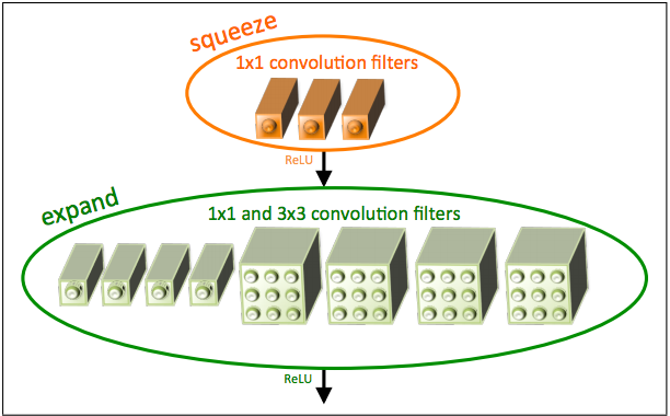
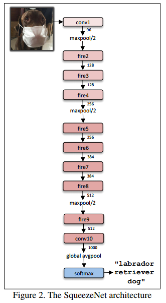
SqueezeNet fire module
|
1 2 3 4 5 6 7 8 9 10 11 12 13 14 15 |
# Squeeze part of fire module with 1 * 1 convolutions, followed by Relu x = Convolution2D(squeeze, (1, 1), padding='valid', name='fire2/squeeze1x1')(x) x = Activation('relu', name='fire2/relu_squeeze1x1')(x) #Expand part has two portions, left uses 1 * 1 convolutions and is called expand1x1 left = Convolution2D(expand, (1, 1), padding='valid', name='fire2/expand1x1')(x) left = Activation('relu', name='fire2/relu_expand1x1')(left) #Right part uses 3 * 3 convolutions and is called expand3x3, both of these are follow#ed by Relu layer, Note that both receive x as input as designed. right = Convolution2D(expand, (3, 3), padding='same', name='fire2/expand3x3')(x) right = Activation('relu', name='fire2/relu_expand3x3')(right) # Final output of Fire Module is concatenation of left and right. x = concatenate([left, right], axis=3, name='fire2/concat') |
We can easily convert this code into a function for reuse:
|
1 2 3 4 5 6 |
sq1x1 = "squeeze1x1" exp1x1 = "expand1x1" exp3x3 = "expand3x3" relu = "relu_" WEIGHTS_PATH = "https://github.com/rcmalli/keras-squeezenet/releases/download/v1.0/squeezenet_weights_tf_dim_ordering_tf_kernels.h5" |
|
1 2 3 4 5 6 7 8 9 10 11 12 13 14 15 16 17 18 19 |
sq1x1 = "squeeze1x1" exp1x1 = "expand1x1" exp3x3 = "expand3x3" relu = "relu_" def fire_module(x, fire_id, squeeze=16, expand=64): s_id = 'fire' + str(fire_id) + '/' x = Convolution2D(squeeze, (1, 1), padding='valid', name=s_id + sq1x1)(x) x = Activation('relu', name=s_id + relu + sq1x1)(x) left = Convolution2D(expand, (1, 1), padding='valid', name=s_id + exp1x1)(x) left = Activation('relu', name=s_id + relu + exp1x1)(left) right = Convolution2D(expand, (3, 3), padding='same', name=s_id + exp3x3)(x) right = Activation('relu', name=s_id + relu + exp3x3)(right) x = concatenate([left, right], axis=3, name=s_id + 'concat') return x |
|
1 2 3 4 5 6 7 8 9 10 11 12 13 14 15 16 17 18 19 20 21 22 23 24 25 |
x = Convolution2D(64, (3, 3), strides=(2, 2), padding='valid', name='conv1')(img_input) x = Activation('relu', name='relu_conv1')(x) x = MaxPooling2D(pool_size=(3, 3), strides=(2, 2), name='pool1')(x) x = fire_module(x, fire_id=2, squeeze=16, expand=64) x = fire_module(x, fire_id=3, squeeze=16, expand=64) x = MaxPooling2D(pool_size=(3, 3), strides=(2, 2), name='pool3')(x) x = fire_module(x, fire_id=4, squeeze=32, expand=128) x = fire_module(x, fire_id=5, squeeze=32, expand=128) x = MaxPooling2D(pool_size=(3, 3), strides=(2, 2), name='pool5')(x) x = fire_module(x, fire_id=6, squeeze=48, expand=192) x = fire_module(x, fire_id=7, squeeze=48, expand=192) x = fire_module(x, fire_id=8, squeeze=64, expand=256) x = fire_module(x, fire_id=9, squeeze=64, expand=256) x = Dropout(0.5, name='drop9')(x) x = Convolution2D(classes, (1, 1), padding='valid', name='conv10')(x) x = Activation('relu', name='relu_conv10')(x) x = GlobalAveragePooling2D()(x) out = Activation('softmax', name='loss')(x) model = Model(inputs, out, name='squeezenet') |
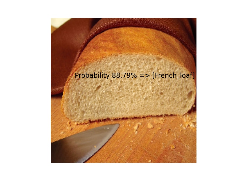
The complete network architecture is defined in squeezenet.py file. We shall download imageNet pre-trained model and run prediction using this model on our own image. Let’s quickly write some code to run this network:
|
1 2 3 4 5 6 7 8 9 10 11 12 13 14 15 16 17 18 |
import numpy as np from keras_squeezenet import SqueezeNet from keras.applications.imagenet_utils import preprocess_input, decode_predictions from keras.preprocessing import image model = SqueezeNet() img = image.load_img('pexels-photo-280207.jpeg', target_size=(227, 227)) x = image.img_to_array(img) x = np.expand_dims(x, axis=0) x = preprocess_input(x) preds = model.predict(x) all_results = decode_predictions(preds) for results in all_results: for result in results: print('Probability %0.2f%% => [%s]' % (100*result[2], result[1])) |
Hopefully, this Keras Tensorflow tutorial gave you a good introduction to Keras. We have learnt:
1. Setting up and installing Keras with Tensorflow Backend.
2. Keras Sequential Models
3. Keras Functional API
4. Saving and loading saved weights in Keras
5. How to solve linear regression using Keras with example code.
As usual, the complete code can be downloaded from our github Repo. You can run all 3 examples by running these 3 files:
|
1 2 3 4 5 6 7 8 9 10 |
#Linear Regression python 1_keras_linear_regression.py # VGG prediction, This downloads 500 MB sized weights # So, it will take a while to run and predict. python 2_run_vgg.py # Squeezenet prediction. The size of pretrained model is 5 MB. Wow! python 3_run_squeezenet.py |
Hopefully, this tutorial helps you in learning Keras with Tensorflow. Do me a favour, if you find this useful, please share with your friends and colleagues who are looking to learn deep learning and computer vision. Happy Learning!
