Unless you have been living under the rock, you must have heard of the revolution that deep learning and convolutional neural networks have brought in computer vision. Computers have achieved near-human level accuracy for most of the tasks. However, most of the top performing neural networks for state of the art image recognition problem suffer from three problems:
1. Low speed:
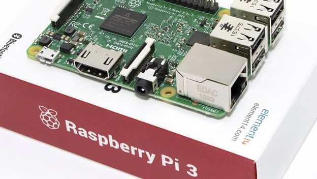
which deter them to get deployed in real time applications on embedded devices like Raspberry PI, Nvidia Jetson etc. This problem gets worse for an application like object detection where multiple windows at different locations and scale need to be processed.
2.Very large model size:
Models that achieve state of the art accuracy are too large to fit into mobile devices or small devices like Raspberry Pi.
3. Large memory footprint:
Even if you somehow manage to live with the large size of models, the amount of run-time memory(RAM) required to run these models is way too high and limits their usage.
Hence, the current trend is to deploy these models on servers with large graphical processing units(GPU), but issues like data privacy and internet connectivity demand usage of embedded deep learning. So huge efforts from people all around the world are geared towards accelerating the inference run-time of these networks, decreasing the size of the model and decreasing the run-time memory requirement.
Why are CNNs slow?
The major chunk of time in a CNN is spent on convolutional layers while the most of the storage is spent on fully connected layers. For example in the AlexNet, 90% of computation time is spent on convolutional layers and 90% of model size is from the weights of FC layers. The newer models like Inception and Resnet have removed the FC layers completely, hence reducing the storage. But still, the models cannot be deployed with low memory footprint. The reason is that during inference, additional memory is utilized for facilitating fast matrix multiplication. Therefore these models can be run on Graphical Processing Units(GPU) with massive memory, but for devices like Raspberry Pi(RAM of 2GB), one has to manage with shallower CNN. Unfortunately, shallower CNNs do not achieve human level accuracy.
So I am planning to publish posts on various strategies for speeding up the CNN and reducing their memory requirements. This particular post is about speeding up the neural network. Let’s get started:
For acceleration convolutional layers of shallow models, a common class of strategy is to decompose weights matrix to save on computation. Acceleration of shallower models is quite an easy problem but for the deeper networks which can match the human accuracy, the same strategies become useless. For deep networks, the speedup for all the layers need to be done simultaneously. If done separately, approximation error of individual layers can get accumulated and significantly affect the accuracy at the last layer, where decision is usually taken place. The following strategy pertains to decomposition of convolutional layers which harnesses the redundancy in parameters and response maps of deep networks. For the VGG model on Imagenet, this method achieves 4X speedup on convolutional layers with only 0.3% increase in top-5 error.
Decomposition of Response Map
A simple method is to decompose layers individually into computationally efficient components. But as mentioned before, this simple trick would render the accumulated error out of hand. So the method described below allows the decomposition of layers in such a way that each layer tries to offset the error accumulated from the layers preceding it.
The idea is that response maps from the CNN are highly redundant and they lie in some lower dimensional subspace which enables convolutional layer to decompose.
Before going further let’s first recap convolution operation.
Convolutional Layer
Lets assume a convolution layer with weight tensor of size d * k * k * c where k is the spatial size of the convolutional kernel, c is the number of input channels and d is the number of filters in the layer. So this whole weight tensor produces d number of neurons with one set of inputs(k * k * c neurons).
Lets consider one filter from this layer which corresponds to k * k * c sized tensor. In the convolution operation, this is element wise multiplied to the input volume of size k * k * c and then summed. A bias term is also added to the resulting summation.
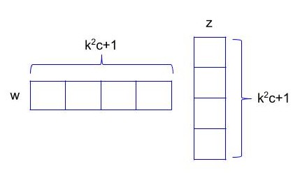
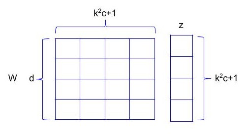
So mathematically let z be the input feature in \(R^{k^{2}c+1}\) and w is the weight associated with one filter. These two are element-wise multiplied and summed to form output neuron.
Now since multiple kernels need to be applied on input, lets arrange these different sets of weights in different rows of a matrix W. So W becomes \(R^{d*k^{2}c+1}\) and output response map would be y = Wz. So y is\(R^{d}\), which is basically a d dimensional vector, same as the number of filters present in the layer.
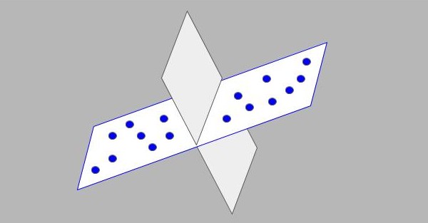
Now imagine a bunch of d dimensional vectors from different images and their different locations. d is typically very large in deep networks and not all the activations are influential in the final prediction implying they are redundant in nature. So let’s assume these d dimensional vectors are actually lying in a lower dimensional space. To have a feel of this, look at the figure 3, where 3-dimensional points are actually residing in a 2-dimensional space corresponding to the plane. So a coordinate system can be obtained with a lower dimension which can accurately approximate the points for the task in hand.
The following analysis is just like PCA, in which the points are first projected into lower dimensional space and then again they are projected back to original space. Obviously, this leads to error, but PCA finds the lower dimensional space such that this error is minimized. If you are familiar with PCA, you can skip the following section.
Lower Rank Subspace
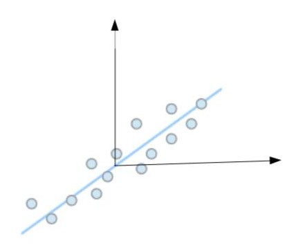
For the sake of convenience, lets take an example with only two dimensional space and random points lying very near to a straight line.
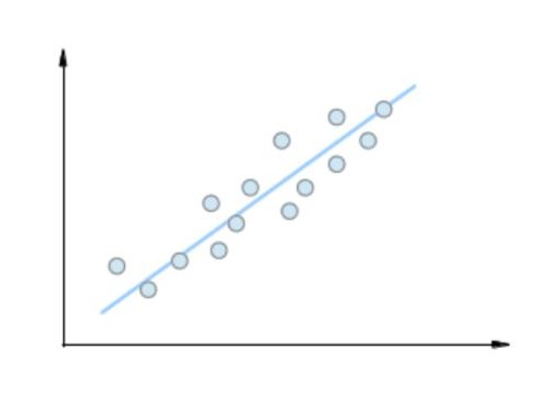
Since along the orthogonal/perpendicular direction to the line, points do not vary much, that direction can be discarded which implies that the two-dimensional space is an overkill for the type of responses we are getting from our layer. If we can somehow get this line, the points can be projected on that line and projected values can be used for further processing. And so one-dimensional representation along the depicted line will be a good approximation to the domain set.
Intuitively the line is the one along which there is maximum variance/spread of the points. And the projection of a vector along a line can be calculated by the dot product between the vector/point and direction of the line. It is similar to calculations for rotating the coordinate system in which a rotation matrix is multiplied to the vector of points to get the vectors in new coordinate system. Now, since rotation matrix does not take translation into account and rotates the vectors by taking origin as the center, so let’s translate the coordinate system to the centroid of the points as depicted in figure.
So \(y_{m}=y-\bar{y}\) , where mean is calculated by taking the mean of all the vectors. Let the line be depicted by v direction vector. Since its a direction vector the l2 norm of v is 1. Projection of a point depicted by \(y_{m,i}\) along this direction is \(v^{T}y^{m,i}\), where i indexes the input vector. Since the mean is zero now, the variance becomes \(\sum_{i=0,n} {(v^{T}y_{m,i}})^{2}\). Here n is the number of input vectors taken into consideration. Lets arrange different y vectors column-wise in a matrix Y. So variance is \(\left\|v^{T}Y\right\|^{2}_{2}\) , the frobenius norm of the matrix formed from each \(y_{m,i}\). In order to get v, the objective becomes:
$$ Maximize \left\|v^{T}Y\right\|^{2}_{2}, subjected to \left\|v\right\|^{2}_{2} = 1 $$
Solving the above constrained equation yields
$$YY^{T}v=\lambda v$$
So the solution for v is eigen vector corresponding to maximum eigen value of the matrix \(YY^{T}\)
Once the vector v representing a direction vector is obtained, any vector/point b can be approximately written as \(vv^{T}b\) where as before \(v^{T}b\) is the projected value on the direction vector.
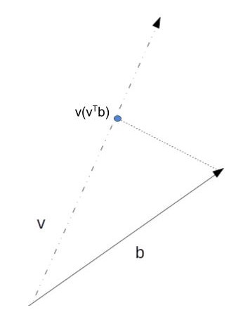
b is a vector/point in n-Dimension space. v is unit vector. Projection of vector b along v is (v^Tb)v
The same methodology can be extended to d dimensional space, wherein the direction of the maximum variance is successively calculated to obtain a sub-space with a pre-defined number of dimensions.
Decomposition
Lets assume we calculated r most effective orthogonal directions where r<d. A matrix V, \(R^{d,r}\) is formed by arranging direction vectors column-wise. Now an approximate version of \(y_{m,i}\), \(\widetilde{y_{m,i}}\) can be obtained by \(VV^{T}y_{m,i}\).
Using equations and doing simple manipulations as shown below, we get a compact formula for y in terms of z.
V is d x r, \(V^{T}\) is r x d and \(\widetilde{y_{m,i}}\) is d x 1.
y from the input to the convolutional layer is Wz,
$$y = Wz $$
$$\widetilde{y_{m}} = VV^{T}y_{m} $$
$$y_{m} = y – \bar{y} $$
$$\widetilde{y_{m}} = VV^{T}Wz – VV^{T}\bar{y}$$
From this approximated mean subtracted vector, the approximated vector is obtained by
$$\widetilde{y} = VV^{T}Wz – VV^{T}\bar{y} + \bar{y}$$
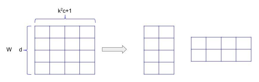
Merging \(V^{T}W\) becomes a new matrix L with dimension r x m. So
$$\widetilde{y} = VLz + b $$
$$b = – VV^{T}\bar{y} + \bar{y}$$
So we have now decomposed the layer into two convolutional layers with weight tensors of V and L. Here b can be taken as bias term for the second convolutional layer.
As evident we have bypassed a large W matrix. So the complexity of calculation has reduced from \(d(k^{2}c+1)\) to \(r(k^{2}c+1)+rd\). r being << d, this significantly reduces the amount of computations.
Also while getting the decomposition of a layer, the inputs are taken as approximated output from preceding layers. This helps to offset error caused by approximation.
A naive approach is to decompose weight tensor W into two lower rank matrices. But that decomposition would not take response maps into account and therefore will be independent of data.
After we are done with decomposing sluggish layers into efficient parts, we can fine-tune the newly formed architecture with the data provided to restore the accuracy lost due to approximation. The paper by Zhang[1] goes further to accommodate the non-linear layer into calculations described above.
The algorithm mentioned has only a 0.3% increase of top-5 error for a 4× speedup on ImageNet classification dataset with VGG model.
References:
- Zhang, Zou, He, Sun: Accelerating Very Deep Convolutional Networks for Classification and Detection
 Since along the orthogonal/perpendicular direction to the line, points do not vary much, that direction can be discarded which implies that the two-dimensional space is an overkill for the type of responses we are getting from our layer. If we can somehow get this line, the points can be projected on that line and projected values can be used for further processing. And so one-dimensional representation along the depicted line will be a good approximation to the domain set.