EfficientNets: The Free lunch of 2019 for convolutional neural networks

Neural network architecture design is one of the key hyperparameters in solving problems using deep learning and computer vision. Various neural networks are compared on two key factors i.e. accuracy and computational requirement. In general, as we aim to design more accurate neural networks, the computational requirement increases.

The term ‘Efficient’ in Efficient Net strongly suggests that this convolutional neural network is the next state-of-the-art network which not only has less number of parameters but also the winner of ILSVRC-2019 with 84.4% and 97.1% as the top-1 and top-5 accuracy respectively. Despite the network has very fewer layers, it has achieved the highest top-1 and top-5 accuracy values in the ImageNet dataset in 2019.

The deep learning researchers are applying their constant effort to find out the best network architecture. The first successful result of the search was AlexNet which achieved 57% as the top-1 accuracy in ILSVRC-2012. Afterward, ZFNet became the champion of ILSVRC-2013. In 2014, the advent of deeper as well as wider network architectures came into existence. VGG and GoogleNet became the champion of ILSVRC-2014. The next winner of ImageNet challenge in ILSVRC-2015 was Deep Residual Network or ResNet. ResNet introduced the skip connections in their network architecture. ResNet was focused to make the architecture as deep as possible. Furthermore, the shortcut connection allowed the gradient to pass in between Residual Blocks so that the vanishing gradient problem for initial layers was rectified. The other networks such as DenseNet-201 and Xception achieved 77.3% and 79% as the top-1 accuracy in the challenge. Also, networks such as NASNet has 88 million parameters achieved 82.5% as the top-1 accuracy. To push the top-1 accuracy value to 84.3%, the giant neural network architecture was built up and named as GPipe. This network has 557M parameters for training. The network is partitioned in 8 parts so that multiple GPU’s can be used to train the network. Training the GPipe network is very complex and this architecture cannot be deployed in a place to solve real-world problems.

How to change the architecture of the network to increase performance?

There can be many ways through which the network architecture can be altered in order to increase the performance. Humans have already put a lot of effort to design the image classifier network architectures manually. Techniques such as Reinforcement Learning is applied to define the search space of the network architectures. In the defined search space, the network architectures are discovered one by one. The discovered architectures are evaluated either by training and validating them on a standard dataset or some mathematical aspects are used to determine the accuracy. The network which gives the highest accuracy on the test set will be selected and can be used for other training purposes.

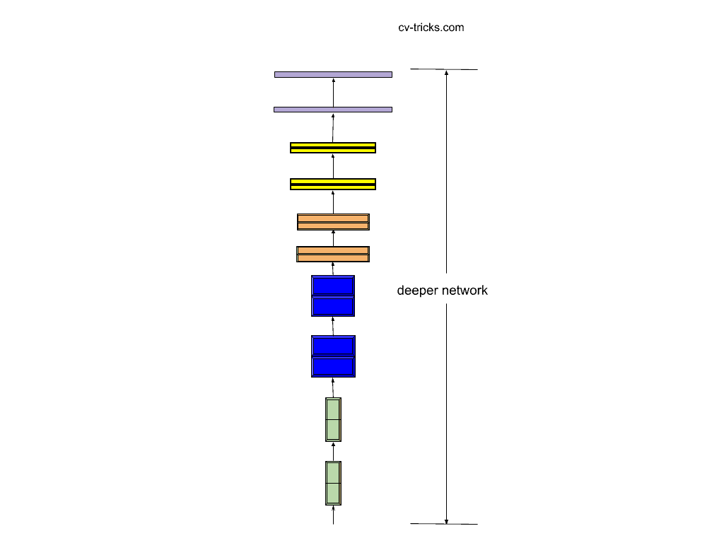
Let’s talk about, what kind of changes can be performed to alter the network architecture. In order to perform the scaling operations, we need to have a good baseline network. The baseline network is as shown below:

Baseline Network to be used for scaling

The traditional CNN’s were scaled arbitrarily with respect to depth. In other words, the number of layers in the network is increased to make it deeper. Deeper networks are able to extract the complex features from the images. These complex features can help the network to increase the classification accuracy. However, the accuracy either saturate or starts to degrade due to the addition of more layers. The reason behind this degradation is the Vanishing Gradient Problem. This problem was addressed with the help of Batch Normalization. Also, ResNets introduced the idea of skip connections which saves the network from vanishing gradient effect. Although the vanishing gradient effect was solved, the network does have a huge number of parameters to be trained. Consequently, training and inference timings will also increase.
Scaling the Baseline w.r.t. Depth
The other method of scaling up the network is to increase the resolution of the input. The high-resolution images contain more pixels i.e. even the simple features in the image are represented using more pixels as compared to less-resolution images. If the detail in the images is increased, then the network will be able to get an increment in the accuracy value. The basic idea behind increasing the resolution of an image will lead to an increase in the depth of the network. We have seen earlier that deeper networks can be used to represent complex features. Therefore, resolution and depth increment may get good accuracy value. But, who knows that at what amount the depth should be increased for the particular increment in the resolution of images. This requires a lot of manual effort and makes the search for optimal architecture as a troublesome process.
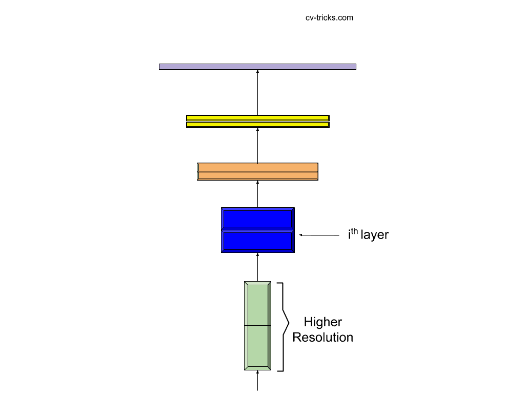
Scaling up the Resolution of the input image.
There is another way to increase the width of the network, i.e. to increase the number of channels along the way to classification. The number of feature maps is increased so as to increase the information being extracted from the image tensors. The wider networks have the capability to represent fine-grained features. The only problem is to figure out the extent to which the network should be made wider to increase the performance. Simply increasing the number of channels will degrade the training speed along with no gain in the classification accuracy value. This also requires manual tuning and good experience with fine-tuning of networks.
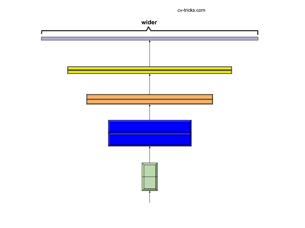
Scaling the width of the baseline network.

Efficient-Net Approach:

The creators of Efficient Net proposed a method known as compound scaling. We have already seen that there are three dimensions in which scaling can be performed to change the network architecture. We can scale either the depth or the width or the resolution of the network. In traditional CNN’s, the scaling was performed with an arbitrary scaling constant in any dimension. The compound scaling suggests that the scaling of the network should be performed using a constant ratio in all the dimensions. The compound scaling method balances all the dimensions of the network i.e width/depth/resolution.

Also, the problem of the extent to which the network should be scaled is solved using the compound scaling technique. The compound scaling makes sense because if the input image is bigger, then the network needs more layers to increase the receptive field and more channels to capture more fine-grained patterns on the bigger image. The general convolutional network is represented as the dot product of image tensor with kernel or feature maps. The network N can be represented as:

N = F_k ☉ …. F_2> ☉ F₁(X₁)

where F_i represents the list of composed layers in the network and X₁ represents the input to the first layer.

or N = _{for i in 1…s}☉ F_i^Li (X< H_i, W_i, C_i> )

where F_i^Li represents that layer F_iis repeated L_i times in stage i. The H_i, W_i, and C_i are scaling coefficients for scaling Height, Width and Channel respectively.

Now, we have to set network length (L_i), network width (C_i) and resolution (H_i , W_i) coefficients to design the network architecture. The final problem can be formulated as follows:

Target: Maximize the Accuracy

_{for d,w,r} max Accuracy(N(d, w, r))

s.t. N(d, w, r) = _{for i in 1…s}☉ F_i^{d * Li} (X< **r * H**_i, r * W_i, w * C_i> )

Memory(N) ≤ target_memory

FLOPS(N) ≤ target_flops

where d, w, and r are the depth, width, and resolution scaling coefficients respectively.

If the network resolution is increased twice that of the original then the amount of computation will be squared to that of the original. The same is the case with increasing the network width. However, increasing the depth of the network will increase the amount of computation in Linear fashion.

Now, the idea of Compound Scaling will be used to increase the network depth, width, and resolution as follows:

Depth: d = 𝛂^Ф

Width: w = β^Ф

Resolution: r = ୪^Ф

s.t. 𝛂 * β² * ୪²≈ 2

where Ф is the user-specific coefficient which controls how many resources are available for model scaling, while 𝛂, β, ୪ specify how to assign these extra resources to network depth, width, and resolution.

Which network should we choose to do scaling?

The network architecture which we will choose for scaling should be good architecture. The meaning of good is that the baseline network architecture should already have achieved decent accuracy value so that further changes can improve it. Therefore, a baseline architecture selection is a very critical point for model scaling. The creators of EfficientNet have done their experiments on some baseline architectures such as ResNet, MobileNet, etc. Furthermore, they have designed their own baseline network using the Neural Architecture Search. Neural Architecture Search uses Reinforcement Learning at its core to design the search space for discovering the new architecture. For example, EfficientNetB0 was designed using the same search space technique used to design MnasNet.

Basic Architecture of EfficientNetB0:

The architecture of EfficientNetB0 is slightly bigger than MnasNet due to the large Floating Point Operations per second target. At the core of EfficientNet, the mobile inverted bottleneck convolution layer is used along with the squeeze and excitation layers. The following table shows the architecture of EfficientNetB0:

Stage i	Operator F_i	Resolution H_i x W_i	# Channels C_i	# Layers L_i
1	Conv 3×3	224 x 224	32	1
2	MBConv1, k-3×3	112 x 112	16	1
3	MBConv6, k-3×3	112 x 112	24	2
4	MBConv6, k-5×5	56 x 56	40	2
5	MBConv6, k-3×3	28 x 28	80	3
6	MBConv6, k-5×5	14 x 14	112	3
7	MBConv6, k-5×5	14 x 14	192	4
8	MBConv6, k-3×3	7 x 7	320	1
9	Conv 1×1 & Pooling & FC	7 x 7	1280	1

The creators of EfficientNet started to scale EfficientNetB0 with the help of their compound scaling method. They applied the grid search technique to get 𝛂 = 1.2, β = 1.1, ୪ = 1.15, Ф = 1. Afterward, they fixed the scaling coefficients and scaled EfficientNetB0 to EfficientNetB7.

Coding the EfficientNet using Keras:

Firstly, we will install the Keras EfficientNet repository into our system. The full code of the repository can be found using this link. To install the repository, run the following command on the terminal:


# Cloning and Installing the Efficient Net Repository
pip install -U git+https://github.com/qubvel/efficientnet

# Cloning and Installing the Efficient Net Repository

pip install -U git+https://github.com/qubvel/efficientnet

The above command will simply clone and install the efficientnet repository. This repository has all the Efficient Net versions i.e. from EfficientNetB0 to EfficientNetB7. Also, this repository provides pre-trained weights on the ImageNet dataset only for EfficentNetB0 to EfficientNetB5. There are no pre-trained weights for EfficientNetB6 and EfficientNetB7. We will show you to train and test EfficientNetB5 using the Cat-Dog classification dataset. The full code of training and testing can be downloaded from this link.


# Import the EfficientNetB5 and other important libraries
from efficientnet import EfficientNetB5
from keras.layers import Dense, GlobalAveragePooling2D
from keras.models import Model
from keras.optimizers import SGD
from keras.preprocessing.image import ImageDataGenerator

# Download the architecture of ResNet50 with ImageNet weights
base_model = EfficientNetB5(weights='imagenet', include_top = False)

# Taking the output of the last layer in EfficientNetB5
x = base_model.output

# Adding a Global Average Pooling layer
x = GlobalAveragePooling2D()(x)

# Adding a fully connected layer having 1000 neurons
x = Dense(1000, activation='relu')(x)

# Adding a fully connected layer having 2 neurons which will
# give probability of image having either dog or cat
predictions = Dense(2, activation='softmax')(x)

# Model to be trained
model = Model(inputs=base_model.input, outputs=predictions)

# Training only top layers i.e. the layers which we have added in the end
for layer in base_model.layers:
    layer.trainable = False

# Compiling the model
model.compile(optimizer=SGD(lr=0.0001, momentum=0.9), loss='categorical_crossentropy', metrics = ['accuracy'])

# Creating objects for image augmentations
train_datagen = ImageDataGenerator(rescale = 1./255,
                                   shear_range = 0.2,
                                   zoom_range = 0.2,
                                   horizontal_flip = True)

test_datagen = ImageDataGenerator(rescale = 1./255)

# Proving the path of training and test dataset
# Setting the image input size as (456, 456)
training_set = train_datagen.flow_from_directory('training_set',
                                                 target_size = (456, 456),
                                                 batch_size = 32,
                                                 class_mode = 'categorical')

test_set = test_datagen.flow_from_directory('test_set',
                                            target_size = (456, 456),
                                            batch_size = 32,
                                            class_mode = 'categorical')

# Training the model for 5 epochs
model.fit_generator(training_set,
                         steps_per_epoch = 8000 // 32,
                         epochs = 5,
                         validation_data = test_set,
                         validation_steps = 2000 // 32)

# Saving the weights in the current directory which can be used later
model.save_weights("Eff_net_weights.h5")

# Setting Up Last Block of EfficientNetB5 to be trainable
for layer in model.layers[-23:]:
	layer.trainable = True

# Compiling the model
model.compile(optimizer=SGD(lr=0.0001, momentum=0.9), loss='categorical_crossentropy', metrics = ['accuracy'])

model.fit_generator(training_set,
                         steps_per_epoch = 8000 // 32,
                         epochs = 5,
                         validation_data = test_set,
                         validation_steps = 2000 // 32)

# Saving the final trained weights in the current directory.
# These weights can be used later to do the inference separately
model.save_weights("Eff_net_final_trained_weights.h5")

# Predicting the final result of image
import numpy as np
from keras.preprocessing import image
test_image = image.load_img('test.jpg', target_size = (456, 456))
test_image = image.img_to_array(test_image)

# Expanding the 3-d image to 4-d image.
# The dimensions will be Batch, Height, Width, Channel
test_image = np.expand_dims(test_image, axis = 0)

# Predicting the final class
result = model.predict(test_image)[0].argmax()

# Fetching the class labels
labels = training_set.class_indices
labels = list(labels.items())

# Printing the final label
for label, i in labels:
    if i == result:
        print("The test image has: ", label)
        break

100

101

102

103

# Import the EfficientNetB5 and other important libraries

from efficientnet import EfficientNetB5

from keras.layers import Dense, GlobalAveragePooling2D

from keras.models import Model

from keras.optimizers import SGD

from keras.preprocessing.image import ImageDataGenerator

# Download the architecture of ResNet50 with ImageNet weights

base_model = EfficientNetB5(weights='imagenet', include_top = False)

# Taking the output of the last layer in EfficientNetB5

x = base_model.output

# Adding a Global Average Pooling layer

x = GlobalAveragePooling2D()(x)

# Adding a fully connected layer having 1000 neurons

x = Dense(1000, activation='relu')(x)

# Adding a fully connected layer having 2 neurons which will

# give probability of image having either dog or cat

predictions = Dense(2, activation='softmax')(x)

# Model to be trained

model = Model(inputs=base_model.input, outputs=predictions)

# Training only top layers i.e. the layers which we have added in the end

for layer in base_model.layers:

layer.trainable = False

# Compiling the model

model.compile(optimizer=SGD(lr=0.0001, momentum=0.9), loss='categorical_crossentropy', metrics = ['accuracy'])

# Creating objects for image augmentations

train_datagen = ImageDataGenerator(rescale = 1./255,

shear_range = 0.2,

zoom_range = 0.2,

horizontal_flip = True)

test_datagen = ImageDataGenerator(rescale = 1./255)

# Proving the path of training and test dataset

# Setting the image input size as (456, 456)

training_set = train_datagen.flow_from_directory('training_set',

target_size = (456, 456),

batch_size = 32,

class_mode = 'categorical')

test_set = test_datagen.flow_from_directory('test_set',

target_size = (456, 456),

batch_size = 32,

class_mode = 'categorical')

# Training the model for 5 epochs

model.fit_generator(training_set,

steps_per_epoch = 8000 // 32,

epochs = 5,

validation_data = test_set,

validation_steps = 2000 // 32)

# Saving the weights in the current directory which can be used later

model.save_weights("Eff_net_weights.h5")

# Setting Up Last Block of EfficientNetB5 to be trainable

for layer in model.layers[-23:]:

layer.trainable = True

# Compiling the model

model.compile(optimizer=SGD(lr=0.0001, momentum=0.9), loss='categorical_crossentropy', metrics = ['accuracy'])

model.fit_generator(training_set,

steps_per_epoch = 8000 // 32,

epochs = 5,

validation_data = test_set,

validation_steps = 2000 // 32)

# Saving the final trained weights in the current directory.

# These weights can be used later to do the inference separately

model.save_weights("Eff_net_final_trained_weights.h5")

# Predicting the final result of image

import numpy as np

from keras.preprocessing import image

test_image = image.load_img('test.jpg', target_size = (456, 456))

test_image = image.img_to_array(test_image)

# Expanding the 3-d image to 4-d image.

# The dimensions will be Batch, Height, Width, Channel

test_image = np.expand_dims(test_image, axis = 0)

# Predicting the final class

result = model.predict(test_image)[0].argmax()

# Fetching the class labels

labels = training_set.class_indices

labels = list(labels.items())

# Printing the final label

for label, i in labels:

if i == result:

print("The test image has: ", label)

break

Results and Key Features of Efficient Net

1- The EfficientNetB7 has achieved 84.4% as top-1 accuracy.

2- EfiicientNetB7 has 66M parameters in total.

3- EfficientNetB0 has 5.5M parameters in total.

References

[1] Mingxing Tan and Quoc V. Le. EfficientNet: Rethinking Model Scaling for Convolutional Neural Networks. ICML 2019. [arxiv]

EfficientNets: The Free lunch of 2019 for convolutional neural networks