Training Image Classification 8x Faster With NFNet

Introduction:

Anyone who has deployed a neural network on production knows that deploying a network is easy but making sure that it stays updated as new user data flows is a harder task. It involves keep training the network with new incoming data frequently and in such a case being able to train faster is very important. In this blog post, we will talk about a new DeepMind paper that describes a new image classification neural network that not only achieves near state of the art accuracy but also can be trained 8 times faster. Of-course this is pretty cool and handy and hence these networks have become very popular. This class of networks are called NF-nets (Normalizer-free networks). This is also a landmark paper because it doesn’t use the batch-normalization which had become de-facto standard for convolutional neural Networks.

Understanding Batch Normalization

Batch normalization is a key component of most image classification models. The vast majority of recent models in computer vision are variants of deep residual networks trained with batch normalization. The combination of these two architectural innovations has enabled practitioners to train significantly deeper networks that can achieve higher accuracies on both the training set and the test set. Before trying to suggest alternatives to batch normalization, one must understand the benefits of batch norm.

1. Batch normalization downscales the residual branch: The combination of skip connections and batch normalization enables us to train significantly deeper networks with thousands of layers. By performing batch norm on the residual branch, we reduce the scale of activation. By scaling down the activations, we avoid exploding gradient problems and get a stable gradient descent early in the training phase.
2. Batch normalization eliminates mean-shift: Activation functions like ReLUs or GELUs, which are not anti-symmetric, have non-zero mean activations. This issue compounds as the network depth increases and introduces a mean shift in the activations, as illustrated in the figure below. This leads to the model predicting a single target class for all training examples. Batch normalization ensures the mean activation on each channel is zero across the current batch, eliminating the mean shift.
   

1. Batch normalization has a regularizing effect: It is widely believed that batch normalization also acts as a regularizer enhancing test set accuracy due to the noise in the batch statistics, which are computed on a subset of the training data.
2. Batch normalization allows efficient large-batch training: Batch normalization smoothens the loss landscape, increasing the largest stable learning rate. While this property does not have practical benefits when the batch size is small, the ability to train at larger learning rates is essential if one wishes to train efficiently with large batch sizes. Large batch training significantly reduces training time because the number of parameter updates is reduced drastically.

Pseudocode for batch normalization

Here, the first step is to calculate the batch mean and variance. The input data is finally normalized before using it as an input to predict y.

Disadvantages of Batch normalization

Batch normalization has three significant practical disadvantages. 

1. It is a surprisingly expensive computational primitive, which incurs memory overhead, and significantly increases the time required to evaluate the gradient in some networks. 
2. It introduces a discrepancy between the model’s behavior during training and at inference time, introducing hidden hyper-parameters that have to be tuned. 
3. Most importantly, batch normalization breaks the independence between training examples in the minibatch. Interaction between training examples may lead to the model being able to “cheat” certain loss functions. 
4. Performance of batch normalized networks decreases when there is high variance within the batch statistics during training. 

Prior Work 

Previously, researchers have tried to eliminate batch normalization by trying to recover one or more benefits of batch normalization. Most of these works suppress the scale of the activations on the residual branch at initialization, by introducing either small constants or learnable scalars. Additionally, it was also observed that the performance of un-normalized deep resnets can be improved by regularization. 

However, recovering 1 or 2 benefits of batch normalization is not sufficient to achieve competitive performance. Hence in this paper, the authors have come up with NF-NETs that are resnets without batch normalization which achieve competitive accuracy. 

Contribution by the NF- Net paper

The authors have come up with a unique training strategy known as adaptive gradient clipping. This clips the gradients of parameters based on the unit-wise ratio of gradient norms to parameter norms. Clipping gradients enable us to train normalizer-free networks with large batch sizes.

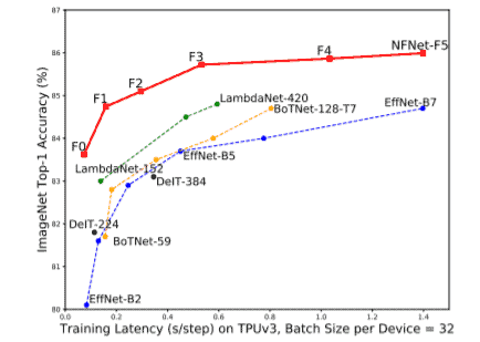
Normalizer-free networks (Nf-nets) have set the new state-of-the-art validation accuracies on Imagenet. As illustrated in figure 1, Nfnet-1 achieves accuracy comparable to effnet-7 whereas nfnet-5 achieves 86.5% accuracy without making use of additional data. 

Adaptive gradient clipping

What is Gradient Clipping?

To train the model at larger batch sizes, various methods of gradient clipping were looked into. Gradient clipping is the process of limiting the gradients at training time to prevent the exploding gradients problem. By limiting the gradient, we put a boundary around the maximum update a parameter can have. In this way, we can stabilize training without batch normalization. Typically, we use the following equation to clip gradients before parameter update

Here, lambda is called clipping threshold. Training stability was extremely sensitive to the choice of the clipping threshold, requiring fine-grained tuning when varying the model depth, the batch size, or the learning rate. The fine-grained tuning required by lambda doesn’t exactly make this method “adaptive”.

What is adaptive gradient clipping?

The motivation behind AGC is a simple observation about the change of parameters during training. We know that while using simple gradient descent without momentum, delta W = – L.r. * G (eqn 1) where W is weights for that layer, LR is learning rate and G is the gradient for that layer. We can say infer the following equation from eqn1 where || . || denotes the Frobenius norm of a matrix. 

We can expect training to destabilize if the LHS of Eqn 2 grows too big since it denotes that there will be huge parameter updates.  

This motivates us to think of a parameter update strategy using clipping which makes use of the ratio in the RHS of eqn 2. In practice, the authors found that unit-wise ratios of gradient norms to parameter norms, performed better empirically than taking layer-wise norm ratios. For more information, you can go through the original paper.

In simpler words, the gradient is clipped according to the ratio of (how large the gradient is)/( how large the parameter on which update will be performed is). 

Results

It was observed that AGC produced robust deep models that can be trained on very strong augmentations too. It was impossible for a normalization-free model without AGC to train on such strong augmentations. 

Furthermore, the AGC enabled NFNET-7 achieved a new state-of-the-art of 86.5% validation accuracy on the imagenet dataset. The previously established effnet-7 had an accuracy of about 84.5% validation accuracy on imagenet. Note that we are comparing this model with effnet-7 since no extra data was used other than imagenet. 

When the above-mentioned model pretrained on a large custom dataset was finetuned on imagenet, it achieved 89% accuracy. 

Furthermore, as shown in the above figure, it was seen that NF-nets without AGC could not be trained on batch sizes larger than a certain threshold. On the other hand, by using AGC we can train our networks on very large batch sizes such as 4096. 

In figure B, it can be seen that the value of lambda is a very sensitive value that must be fine-tuned according to the model and batch size. As you can see, on larger batch sizes, increasing the threshold leads to unstable training.