In some previous tutorials, we learned how to build image classifiers using convolutional neural networks or build object detectors using CNNs. In both examples, all the information required to identify the dog or cat is present in the image.

However, there are many use-cases where the current prediction not only depends on the current input but also on a historical input as well. Have a look at the keyboard on your mobile, the automatic prediction depends on what have we written so far.

Similarly, in a video, we can use the information from the previous frames to predict the output of the current frame. In all of these examples, we use historical data to improve our current prediction. That’s where we use RNNs or Recurrent neural networks.
Similarly, RNNs can be used to describe the content of an image:
One of the most popular implementations of Deep Learning or Machine Learning for that matter has been pattern recognition. An example of the aforementioned paradigm is predicting the future output of a time series given some historical data.
RNNs, short for Recurrent Neural Network help us solve problems that involve time-series datasets. A classic example of RNNs in place would be the auto-suggest feature in smartphones. The model suggests the next word in the sentence given the input that has been fed into it over time. But how do these models work?
Contrary to the traditional neural networks, which take a fixed set of inputs into a framework and output a vector of fixed space, RNNs take in sequences of vectors and give an output, which itself is used as an input feature for future inputs. Confused?
This is a classical neuron. It takes in input, does a weighted sum on it, and passes it through an activation function to give an output of fixed shape.


This represents a typical RNN neuron.

The data entering the neuron is not singular but is a series of data points entering in a specific order. Consider a single data point Xt, the output corresponding to the data point, ht is fed back into the neuron as an input for the next data point ie.. ht+1. This means that in theory, while computing an output for Xt, the neuron also considers the output of ht-1 which in turn implies that ht+1 depends on ht which in turn also depends on ht-1 just like in recursion, hence the name.
Next to the figure of the RNN neuron is an unrolled representation of the same to help you understand better.


1st model is a traditional neural network, while the others are types of RNNs. 2. Vector to Sequence 3. Sequence to Vector 4,5. Sequence to Sequence
So what makes RNNs so powerful?
RNNs use historical time series data to model their weights which finds use in many interesting Machine Learning problems like predicting Stock Prices, Future Production, Audio/Video processing, Speech Recognition, etc. Even Google’s famous A.I. Game Quick Draw uses an RNN to predict the doodles modeling the way the doodle is drawn.
RNNs are Turing Complete in a way, ie. an RNN architecture can be used to approximate arbitrary programs, theoretically, given proper weights, which naturally leads to more intelligent systems. Of course, RNNs are not practically Turing Complete for all problems given that making the input/output vector large can slow the RNN significantly.
Which brings us to the next part of this Article, LSTMs
A Recurrent Neural Network using classical neurons gets slower as the size of size time-series input increases. A solution to this can be limiting the number of data points in a single batch during training, but doing this means that our model would not be able to utilize the information spread over large intervals. For example, If you’re trying to design an RNN which predicts the next word in the sentence, the RNN model would not have much difficulty in suggesting “sky” given the input “Birds fly high in the big blue” because the context that connects the given sentence to the word “sky” ie… words like “blue”,” fly” occur close to the given target. However, for a Sentence like “I was born in India. My parents, as well as my grandparents, lived here. The culture is very rich herein ”, the model would not be able to predict the word “India” simply because the model has not been trained to identify contexts over such a long data sequence.


Context closer to the target is picked easily


The solution to the above problems was given in 1997 when a research paper introduced the world to the concept of Long Short term memory through LSTM Cells. The paper was written considering Sepp Hochreiter’s analysis of the Fundamental Deep Learning Problem dated 1991. In his analysis, Hochreiter discussed issues with Deep Learning, like Vanishing and Exploding gradients which were later solved using better activation functions, like RELU and techniques like Gradient Chopping et all, LSTMs being one of the solutions to the presented problems.
So what is LSTM all about, and how does it solve our problem?
The diagram illustrated below really drives our point home. The cell shown above is a normal cell with a tanh activation function, while the one below is an LSTM cell. Now there is a lot going on inside an LSTM Cell, and it requires a separate analysis.


Normal RNN Cell vs LSTM cell
Look at the diagram given below,

LSTM Cell
LSTM cells are specifically designed to hold information through the chain of neurons to ensure that the relevant data stays through the network without the need to actually store the complete data sequence.
In the diagram above, Xt is the data point at time t, ht-1 is the output of the network at t-1 and Ct is the special storage unit exclusive to the LSTM called Cell State, this is where the magic happens. You can think of a Ct as a buffer that stores data through the network to ensure that relevant data is not lost or forgotten.
Let’s look at what goes on inside an LSTM cell.
The cell takes in Xt and ht-1 and applies an activation on the two to output ft called the forget layer, which ranges between 0 and 1(since the activation used here is sigmoid). ft represents the fraction of the Ct-1 that needs to be forgotten in the view of new data that enters the network. Here 1 represents that all of the previous data needs to be forgotten while 0 means that all of the previous data needs to be retained. For example, in the auto-suggest program, if Ct-1 currently stores the pronoun of a character in the text being input, but at time t, Xt introduces a new character, the previous pronoun needs to let go. This is done by applying ft on Ct-1.


Next comes the the it and C̃t layer which is basically an update to the Cell State, all the new information to be added to the cell state goes through this layer.
The sigmoid layer creates it which is called input gate layer, it represents the fraction of information to be added to the Cell State. The tanh layer creates C̃t which is basically a vector of Candidate Values which can be added to the cell state. The it and C̃t layer are combined to create an update to the cell state depending on the fraction of each candidate value to be updated, which is determined through it.


Combining the two previous steps, we get the new cell state which emerges after forgetting the irrelevant part, through ft*Ct-1 and updating new values through it*C̃t


Next, we need to define the output of the LSTM cell. Now keep in mind that we need to produce an output while keeping in mind the previous information, stored in the cell state and the new information fed to the cell i.e. Xt and ht-1.
The new information is passed through a sigmoid filter that creates an output layer ot this output layer is combined with the updated cell state Ct passed through a tanh activation function to give the cell’s output ie.. ht. For example.. In auto complete, if the model encounters a new subject, it would output a verb or relevant word keeping in mind the information updated about the subject in the cell state and the new data point added to the model.


What we just witnessed was an LSTM cell, there are several alternatives to the LSTM cells like the recently introduced Gated Recurrent Units (GRUs) 2014. GRUs merge the forget and input layers into a single update layer thereby simplifying the process.


These were the two most popular RNN cells, there are many variants of LSTMs with slight changes in the cell structure, each suitable for specific tasks.
Now that we have a basic understanding of what RNNs are and how the memory cells work, let’s look at a vanilla RNN example implemented in Python and Numpy.
For the sake of this example, we will be using Andrej Karpathy’s minimal character-level language model available here.
But for a better understanding of how the model works and to get some significant results from the model, we will be altering the code to train on a simpler dataset than character series. We will make an RNN regression model which will predict the value of cos(x) given some historical seed data.
Let’s jump to the code.
|
1 2 3 4 5 6 7 8 9 10 11 12 13 14 15 16 17 18 19 |
class data(): def __init__(self,x_min,x_max,num_points): self.xmin = x_min self.xmax = x_max self.num_points = num_points self.resolution = (self.xmax-self.xmin)/self.num_points self.x_data = np.linspace(self.xmin,self.xmax,num_points) self.y_true = np.cos(self.x_data) + np.random.normal(size=self.x_data.shape)*0.05 def next_batch(self,steps,return_batch_x=False): rand_start = np.random.rand(1) rand_start = rand_start * (self.xmax- self.xmin - ((steps+1)*self.resolution) ) x_batch = rand_start + np.arange(0,steps+1)*self.resolution y_batch = np.cos(x_batch) #print(x_batch) if(return_batch_x==True): return y_batch[:-1], y_batch[1:] ,x_batch else: return y_batch[:-1], y_batch[1:] |
Data Class
First we create a data class, this will be used to create and manage data for training and testing purposes. The class returns an instance storing the cos function based on the inputs given to it. For the sake of generalization, we have added some random noise to the data given by
np.random.normal(size=self.x_data.shape)*0.05
This is how the training data looks like. We can see obvious trends in this data, let’s see if our RNN model is able to see the same.
The class also has a function called next_batch, which returns batches of data for training purposes. It takes in a variable called steps. This variable determines the number of training points will the model evaluate the loss on each iteration. The function takes a random start point on the x-axis(within the given range) and samples steps+1 points on it. It then calculates the corresponding y values. So if the number of steps in a model is 20, then the batch has two arrays each containing 21 values. The function returns two arrays(or three is the model needs the x values as well), one being the first 20 values, this is the input vector, which goes into the RNN, other being the last 20 values, this is the target. Out network will take in the input vector and return the predicted value for each element in the input vector. These values will be compared to the corresponding values in the target vector. The model will adjust parameters to minimize the difference between these values, in a way teaching it to predict the next cos value when a single cos value is available.
Model Architecture
|
1 2 3 4 5 6 7 8 9 10 11 12 13 14 15 16 17 18 19 20 21 22 23 |
train_data = data(0,100,10000) # hyperparameters hidden_size = 100 # size of hidden layer of neurons learning_rate = 0.001 input_size = 1 #because in this case, the model has to predict the value of the next output, not probability step_size = 50 training_steps = 100000 # batch_size = 1 output_size = 1 # model parameters Wxh = np.random.randn(hidden_size, input_size)*0.01 # input to hidden Whh = np.random.randn(hidden_size, hidden_size)*0.01 # hidden to hidden Why = np.random.randn(output_size, hidden_size)*0.01 # hidden to output bh = np.zeros((hidden_size, 1)) # hidden bias by = np.zeros((output_size, 1)) # output bias p = 0 hprev = np.zeros((hidden_size,1)) # reset RNN memory mWxh, mWhh, mWhy = np.zeros_like(Wxh), np.zeros_like(Whh), np.zeros_like(Why)# memory variables for Adagrad mbh, mby = np.zeros_like(bh), np.zeros_like(by) loss_map = [] |
The model consists of a single hidden layer and a single memory layer hprev.
It takes in a single float value as input outputs a single float value. At the start of training, the RNN memory is reset to zeros, this memory cell will store information as the training proceeds.
Apart from weights and biases, the model also has a memory variable which will be used later for the Adagrad optimization algorithm.
To understand how the model calculates the predicted value, let’s have a look at the loss function.
|
1 2 3 4 5 6 7 8 9 10 11 12 13 14 15 16 17 18 19 20 21 22 23 24 25 26 27 28 29 30 31 32 33 34 35 36 37 38 |
def lossFun(inputs, targets, hprev,Wxh,Whh,Why,bh,by): """ inputs,targets are both arrays of floats. hprev is Hx1 array of initial hidden state returns the loss, gradients on model parameters, and last hidden state """ xs, hs, ys = {}, {}, {} hs[-1] = np.copy(hprev) loss = 0 # forward pass for t in range(len(inputs)): xs[t] = inputs[t] hs[t] = np.tanh(np.dot(Wxh, xs[t]) + np.dot(Whh, hs[t-1]) + bh) # hidden state ys[t] = np.dot(Why, hs[t]) + by # output of the network #ps[t] = np.exp(ys[t]) / np.sum(np.exp(ys[t])) # probabilities for next chars loss += np.square(ys[t][0][0]-targets[t]) #loss += -np.log(ps[t][targets[t],0]) # softmax (cross-entropy loss) loss /= 2*len(inputs) #print(loss) # backward pass: compute gradients going backwards dWxh, dWhh, dWhy = np.zeros_like(Wxh), np.zeros_like(Whh), np.zeros_like(Why) dbh, dby = np.zeros_like(bh), np.zeros_like(by) dhnext = np.zeros_like(hs[0]) for t in reversed(range(len(inputs))): dy = np.copy(ys[t]) dy[0][0] -= targets[t] # backprop into y. see http://cs231n.github.io/neural-networks-case-study/#grad if confused here dWhy += np.dot(dy, hs[t].T) dby += dy dh = np.dot(Why.T, dy) + dhnext # backprop into h dhraw = (1 - hs[t] * hs[t]) * dh # backprop through tanh nonlinearity dbh += dhraw dWxh += np.dot(dhraw, xs[t].T) dWhh += np.dot(dhraw, hs[t-1].T) dhnext = np.dot(Whh.T, dhraw) for dparam in [dWxh, dWhh, dWhy, dbh, dby]: np.clip(dparam, -5, 5, out=dparam) # clip to mitigate exploding gradients return loss, dWxh, dWhh, dWhy, dbh, dby, hs[len(inputs)-1] |
The loss function has been taken as it is, with some minor changes. xs, hs, ys are dictionaries to keep track of inputs, hidden states, and outputs respectively. Since the output of an input t depends on xs[t] as well as hs[t-1], hs needs to have some initial value, which is given by the memory cell of the network, hprev.
xs[t] = inputs[t] initializes the input value in the dictionary
hs[t] = np.tanh(np.dot(Wxh, xs[t]) + np.dot(Whh, hs[t-1]) + bh) computes the hidden layer of the network. Notice that it depends on both the input value as well has the hidden layer of the previous input.
ys[t] = np.dot(Why, hs[t]) + by computes the output of the network.
This output is then used to calculate the loss. We are using the mean square loss function in this case.
The function then uses backpropagation to calculate the gradients of the weights and biases.
In the end, the function returns the loss, gradients, and the memory cell ie.. the last element of the hs dictionary.
|
1 2 3 4 |
for param, dparam, mem in zip([Wxh, Whh, Why, bh, by],[dWxh, dWhh, dWhy, dbh, dby],[mWxh, mWhh, mWhy, mbh, mby]): mem += dparam * dparam param += -learning_rate * dparam / np.sqrt(mem + 1e-8) # adagrad update |
This single line then makes an update to the weights and biases through the adagrad upgrade.
Running the model for the given number of iterations with say 20 as the number of steps, the model randomly chooses 21 points from the dataset and makes an update to the weights and biases for iteration.
After training this model for 100000 training steps with a relatively small learning rate of 0.001, we get this loss function.

Here are some of the test outputs, notice how we used a smooth cos function for test input to make sure that the model is able to generalize well.


Credits:
1. Christopher Olah’s Blog for these awesome diagrams
2. Andrej Karpathy’s Minimal Character-Level Language Model for the base code.